Make MTH5 from IRIS Data Managment Center v0.2.0
This example demonstrates how to build an MTH5 from data archived at IRIS, it could work with any MT data stored at an FDSN data center (probably).
We will use the mth5.clients.FDSN class to build the file. There is also second way using the more generic mth5.clients.MakeMTH5 class, which will be highlighted below.
Note: this example assumes that data availability (Network, Station, Channel, Start, End) are all previously known. If you do not know the data that you want to download use IRIS tools to get data availability.
[1]:
from pathlib import Path

import numpy as np
import pandas as pd
from mth5.mth5 import MTH5
from mth5.clients.make_mth5 import FDSN, MakeMTH5

from matplotlib import pyplot as plt
%matplotlib widget
Set the path to save files to as the current working directory
[2]:
default_path = Path().cwd()
Initialize a MakeMTH5 object
Here, we are setting the MTH5 file version to 0.2.0 so that we can have multiple surveys in a single file. Also, setting the client to “IRIS”. Here, we are using obspy.clients tools for the request. Here are the available FDSN clients.
Note: Only the “IRIS” client has been tested.
[3]:
fdsn_object = FDSN(mth5_version='0.2.0')
fdsn_object.client = "IRIS"
Make the data inquiry as a DataFrame
There are a few ways to make the inquiry to request data.
Make a DataFrame by hand. Here we will make a list of entries and then create a DataFrame with the proper column names
You can create a CSV file with a row for each entry. There are some formatting that you need to be aware of. That is the column names and making sure that date-times are YYYY-MM-DDThh:mm:ss
Column Name |
Description |
|---|---|
network |
|
station |
|
location |
|
channel |
|
start |
Start time (YYYY-MM-DDThh:mm:ss) UTC |
end |
End time (YYYY-MM-DDThh:mm:ss) UTC |
[4]:
channels = ["LFE", "LFN", "LFZ", "LQE", "LQN"]
CAS04 = ["8P", "CAS04",  '2020-06-02T19:00:00', '2020-07-13T19:00:00']
NVR08 = ["8P", "NVR08", '2020-06-02T19:00:00', '2020-07-13T19:00:00']
# REV06 = ["8P", "REV06", '2020-06-02T19:00:00', '2020-07-13T19:00:00']

stations = [CAS04, NVR08,]
# stations.append(REV06)

request_list = []
for entry in stations:
    for channel in channels:
        request_list.append(
            [entry[0], entry[1], "", channel, entry[2], entry[3]]
        )

# Turn list into dataframe
request_df =  pd.DataFrame(request_list, columns=fdsn_object.request_columns)
request_df
[4]:
| network | station | location | channel | start | end | |
|---|---|---|---|---|---|---|
| 0 | 8P | CAS04 | LFE | 2020-06-02T19:00:00 | 2020-07-13T19:00:00 | |
| 1 | 8P | CAS04 | LFN | 2020-06-02T19:00:00 | 2020-07-13T19:00:00 | |
| 2 | 8P | CAS04 | LFZ | 2020-06-02T19:00:00 | 2020-07-13T19:00:00 | |
| 3 | 8P | CAS04 | LQE | 2020-06-02T19:00:00 | 2020-07-13T19:00:00 | |
| 4 | 8P | CAS04 | LQN | 2020-06-02T19:00:00 | 2020-07-13T19:00:00 | |
| 5 | 8P | NVR08 | LFE | 2020-06-02T19:00:00 | 2020-07-13T19:00:00 | |
| 6 | 8P | NVR08 | LFN | 2020-06-02T19:00:00 | 2020-07-13T19:00:00 | |
| 7 | 8P | NVR08 | LFZ | 2020-06-02T19:00:00 | 2020-07-13T19:00:00 | |
| 8 | 8P | NVR08 | LQE | 2020-06-02T19:00:00 | 2020-07-13T19:00:00 | |
| 9 | 8P | NVR08 | LQN | 2020-06-02T19:00:00 | 2020-07-13T19:00:00 |
Save the request as a CSV
Its helpful to be able to save the request as a CSV and modify it and use it later. A CSV can be input as a request to MakeMTH5
[5]:
request_df.to_csv(default_path.joinpath("fdsn_request.csv"))
Get only the metadata from IRIS
It can be helpful to make sure that your request is what you would expect. For that you can request only the metadata from IRIS. The request is quick and light so shouldn’t need to worry about the speed. This returns a StationXML file and is loaded into an obspy.Inventory object.
[6]:
inventory, data = fdsn_object.get_inventory_from_df(request_df, data=False)
Have a look at the Inventory to make sure it contains what is requested.
[7]:
inventory
[7]:
Inventory created at 2024-08-10T00:27:45.912403Z
        Created by: ObsPy 1.4.0
                    https://www.obspy.org
        Sending institution: MTH5
        Contains:
                Networks (1):
                        8P
                Stations (2):
                        8P.CAS04 (Corral Hollow, CA, USA)
                        8P.NVR08 (Rhodes Salt Marsh, NV, USA)
                Channels (13):
                        8P.CAS04..LFZ, 8P.CAS04..LFN, 8P.CAS04..LFE, 8P.CAS04..LQN (2x),
                        8P.CAS04..LQE (3x), 8P.NVR08..LFZ, 8P.NVR08..LFN, 8P.NVR08..LFE,
                        8P.NVR08..LQN, 8P.NVR08..LQE
Make an MTH5 from a request
Now that we’ve created a request, and made sure that its what we expect, we can make an MTH5 file. The input can be either the DataFrame or the CSV file.
We are going to time it just to get an indication how long it might take. Should take about 4 minutes.
Note: we are setting interact=False. If you want to just to keep the file open to interrogate it set interact=True. Then an MTH5 object would be returned instead of the path to the mth5 file.
Make an MTH5 using MakeMTH5
Another way to make a file is using the mth5.clients.MakeMTH5 class, which is more generic than FDSN, but doesn’t have as many methods. The MakeMTH5 class is meant to be a convienence method for the various clients.
from mth5.clients import MakeMTH5

make_mth5_object = MakeMTH5(mth5_version='0.2.0', interact=False)
mth5_filename = make_mth5_object.from_fdsn_client(request_df, client="IRIS")
[8]:
%%time

mth5_filename = MakeMTH5.from_fdsn_client(request_df, interact=False)

print(f"Created {mth5_filename}")
2024-08-09T17:27:46.822659-0700 | WARNING | mth5.mth5 | open_mth5 | 8P_CAS04_NVR08.h5 will be overwritten in 'w' mode
2024-08-09T17:27:47.121253-0700 | INFO | mth5.mth5 | _initialize_file | Initialized MTH5 0.2.0 file /home/kkappler/software/irismt/mth5/docs/examples/notebooks/8P_CAS04_NVR08.h5 in mode w
2024-08-09T17:28:18.046696-0700 | INFO | mt_metadata.timeseries.filters.filtered | _check_consistency | Assuming all filters have been applied as True
2024-08-09T17:28:18.090356-0700 | INFO | mt_metadata.timeseries.filters.filtered | _check_consistency | Assuming all filters have been applied as True
2024-08-09T17:28:18.148235-0700 | INFO | mt_metadata.timeseries.filters.filtered | _check_consistency | Assuming all filters have been applied as True
2024-08-09T17:28:18.167371-0700 | INFO | mt_metadata.timeseries.filters.obspy_stages | create_filter_from_stage | Converting PoleZerosResponseStage electric_si_units to a CoefficientFilter.
2024-08-09T17:28:18.181537-0700 | INFO | mt_metadata.timeseries.filters.obspy_stages | create_filter_from_stage | Converting PoleZerosResponseStage electric_dipole_92.000 to a CoefficientFilter.
2024-08-09T17:28:18.233418-0700 | INFO | mt_metadata.timeseries.filters.filtered | _check_consistency | Assuming all filters have been applied as True
2024-08-09T17:28:18.247676-0700 | INFO | mt_metadata.timeseries.filters.obspy_stages | create_filter_from_stage | Converting PoleZerosResponseStage electric_si_units to a CoefficientFilter.
2024-08-09T17:28:18.262440-0700 | INFO | mt_metadata.timeseries.filters.obspy_stages | create_filter_from_stage | Converting PoleZerosResponseStage electric_dipole_92.000 to a CoefficientFilter.
2024-08-09T17:28:18.316113-0700 | INFO | mt_metadata.timeseries.filters.filtered | _check_consistency | Assuming all filters have been applied as True
2024-08-09T17:28:18.327193-0700 | INFO | mt_metadata.timeseries.filters.obspy_stages | create_filter_from_stage | Converting PoleZerosResponseStage electric_si_units to a CoefficientFilter.
2024-08-09T17:28:18.338572-0700 | INFO | mt_metadata.timeseries.filters.obspy_stages | create_filter_from_stage | Converting PoleZerosResponseStage electric_dipole_92.000 to a CoefficientFilter.
2024-08-09T17:28:18.384337-0700 | INFO | mt_metadata.timeseries.filters.filtered | _check_consistency | Assuming all filters have been applied as True
2024-08-09T17:28:18.388468-0700 | INFO | mt_metadata.timeseries.filters.obspy_stages | create_filter_from_stage | Converting PoleZerosResponseStage electric_si_units to a CoefficientFilter.
2024-08-09T17:28:18.396824-0700 | INFO | mt_metadata.timeseries.filters.obspy_stages | create_filter_from_stage | Converting PoleZerosResponseStage electric_dipole_92.000 to a CoefficientFilter.
2024-08-09T17:28:18.436229-0700 | INFO | mt_metadata.timeseries.filters.filtered | _check_consistency | Assuming all filters have been applied as True
2024-08-09T17:28:18.446385-0700 | INFO | mt_metadata.timeseries.filters.obspy_stages | create_filter_from_stage | Converting PoleZerosResponseStage electric_si_units to a CoefficientFilter.
2024-08-09T17:28:18.455777-0700 | INFO | mt_metadata.timeseries.filters.obspy_stages | create_filter_from_stage | Converting PoleZerosResponseStage electric_dipole_92.000 to a CoefficientFilter.
2024-08-09T17:28:18.497077-0700 | INFO | mt_metadata.timeseries.filters.filtered | _check_consistency | Assuming all filters have been applied as True
2024-08-09T17:28:18.541725-0700 | INFO | mt_metadata.timeseries.filters.filtered | _check_consistency | Assuming all filters have been applied as True
2024-08-09T17:28:18.571912-0700 | INFO | mt_metadata.timeseries.filters.filtered | _check_consistency | Assuming all filters have been applied as True
2024-08-09T17:28:18.604210-0700 | INFO | mt_metadata.timeseries.filters.filtered | _check_consistency | Assuming all filters have been applied as True
2024-08-09T17:28:18.611862-0700 | INFO | mt_metadata.timeseries.filters.obspy_stages | create_filter_from_stage | Converting PoleZerosResponseStage electric_si_units to a CoefficientFilter.
2024-08-09T17:28:18.620346-0700 | INFO | mt_metadata.timeseries.filters.obspy_stages | create_filter_from_stage | Converting PoleZerosResponseStage electric_dipole_94.000 to a CoefficientFilter.
2024-08-09T17:28:18.667059-0700 | INFO | mt_metadata.timeseries.filters.filtered | _check_consistency | Assuming all filters have been applied as True
2024-08-09T17:28:18.679981-0700 | INFO | mt_metadata.timeseries.filters.obspy_stages | create_filter_from_stage | Converting PoleZerosResponseStage electric_si_units to a CoefficientFilter.
2024-08-09T17:28:18.689536-0700 | INFO | mt_metadata.timeseries.filters.obspy_stages | create_filter_from_stage | Converting PoleZerosResponseStage electric_dipole_94.000 to a CoefficientFilter.
2024-08-09T17:28:18.736415-0700 | INFO | mt_metadata.timeseries.filters.filtered | _check_consistency | Assuming all filters have been applied as True
2024-08-09T17:28:19.499236-0700 | INFO | mt_metadata.timeseries.filters.filtered | _check_consistency | Assuming all filters have been applied as True
2024-08-09T17:28:19.501143-0700 | INFO | mt_metadata.timeseries.filters.filtered | _check_consistency | Assuming all filters have been applied as True
2024-08-09T17:28:19.503082-0700 | INFO | mt_metadata.timeseries.filters.filtered | _check_consistency | Assuming all filters have been applied as True
2024-08-09T17:28:19.505166-0700 | INFO | mt_metadata.timeseries.filters.filtered | _check_consistency | Assuming all filters have been applied as True
2024-08-09T17:28:19.506926-0700 | INFO | mt_metadata.timeseries.filters.filtered | _check_consistency | Assuming all filters have been applied as True
2024-08-09T17:28:19.533889-0700 | INFO | mt_metadata.timeseries.filters.filtered | _check_consistency | Assuming all filters have been applied as True
2024-08-09T17:28:19.535791-0700 | INFO | mt_metadata.timeseries.filters.filtered | _check_consistency | Assuming all filters have been applied as True
2024-08-09T17:28:19.537838-0700 | INFO | mt_metadata.timeseries.filters.filtered | _check_consistency | Assuming all filters have been applied as True
2024-08-09T17:28:19.539704-0700 | INFO | mt_metadata.timeseries.filters.filtered | _check_consistency | Assuming all filters have been applied as True
2024-08-09T17:28:19.541825-0700 | INFO | mt_metadata.timeseries.filters.filtered | _check_consistency | Assuming all filters have been applied as True
2024-08-09T17:28:19.573254-0700 | INFO | mt_metadata.timeseries.filters.filtered | _check_consistency | Assuming all filters have been applied as True
2024-08-09T17:28:19.575574-0700 | INFO | mt_metadata.timeseries.filters.filtered | _check_consistency | Assuming all filters have been applied as True
2024-08-09T17:28:19.577376-0700 | INFO | mt_metadata.timeseries.filters.filtered | _check_consistency | Assuming all filters have been applied as True
2024-08-09T17:28:19.579105-0700 | INFO | mt_metadata.timeseries.filters.filtered | _check_consistency | Assuming all filters have been applied as True
2024-08-09T17:28:19.580888-0700 | INFO | mt_metadata.timeseries.filters.filtered | _check_consistency | Assuming all filters have been applied as True
2024-08-09T17:28:19.610052-0700 | INFO | mt_metadata.timeseries.filters.filtered | _check_consistency | Assuming all filters have been applied as True
2024-08-09T17:28:19.612148-0700 | INFO | mt_metadata.timeseries.filters.filtered | _check_consistency | Assuming all filters have been applied as True
2024-08-09T17:28:19.614064-0700 | INFO | mt_metadata.timeseries.filters.filtered | _check_consistency | Assuming all filters have been applied as True
2024-08-09T17:28:19.615663-0700 | INFO | mt_metadata.timeseries.filters.filtered | _check_consistency | Assuming all filters have been applied as True
2024-08-09T17:28:19.617472-0700 | INFO | mt_metadata.timeseries.filters.filtered | _check_consistency | Assuming all filters have been applied as True
2024-08-09T17:28:20.105410-0700 | INFO | mt_metadata.timeseries.filters.filtered | _check_consistency | Assuming all filters have been applied as True
2024-08-09T17:28:20.107615-0700 | INFO | mt_metadata.timeseries.filters.filtered | _check_consistency | Assuming all filters have been applied as True
2024-08-09T17:28:20.109495-0700 | INFO | mt_metadata.timeseries.filters.filtered | _check_consistency | Assuming all filters have been applied as True
2024-08-09T17:28:20.111962-0700 | INFO | mt_metadata.timeseries.filters.filtered | _check_consistency | Assuming all filters have been applied as True
2024-08-09T17:28:20.113690-0700 | INFO | mt_metadata.timeseries.filters.filtered | _check_consistency | Assuming all filters have been applied as True
2024-08-09T17:28:20.140969-0700 | INFO | mt_metadata.timeseries.filters.filtered | _check_consistency | Assuming all filters have been applied as True
2024-08-09T17:28:20.143112-0700 | INFO | mt_metadata.timeseries.filters.filtered | _check_consistency | Assuming all filters have been applied as True
2024-08-09T17:28:20.144985-0700 | INFO | mt_metadata.timeseries.filters.filtered | _check_consistency | Assuming all filters have been applied as True
2024-08-09T17:28:20.146871-0700 | INFO | mt_metadata.timeseries.filters.filtered | _check_consistency | Assuming all filters have been applied as True
2024-08-09T17:28:20.148753-0700 | INFO | mt_metadata.timeseries.filters.filtered | _check_consistency | Assuming all filters have been applied as True
2024-08-09T17:28:20.176227-0700 | INFO | mt_metadata.timeseries.filters.filtered | _check_consistency | Assuming all filters have been applied as True
2024-08-09T17:28:20.178456-0700 | INFO | mt_metadata.timeseries.filters.filtered | _check_consistency | Assuming all filters have been applied as True
2024-08-09T17:28:20.180312-0700 | INFO | mt_metadata.timeseries.filters.filtered | _check_consistency | Assuming all filters have been applied as True
2024-08-09T17:28:20.182088-0700 | INFO | mt_metadata.timeseries.filters.filtered | _check_consistency | Assuming all filters have been applied as True
2024-08-09T17:28:20.185302-0700 | INFO | mt_metadata.timeseries.filters.filtered | _check_consistency | Assuming all filters have been applied as True
2024-08-09T17:28:20.352798-0700 | INFO | mt_metadata.timeseries.filters.filtered | _check_consistency | Assuming all filters have been applied as True
2024-08-09T17:28:20.354684-0700 | INFO | mt_metadata.timeseries.filters.filtered | _check_consistency | Assuming all filters have been applied as True
2024-08-09T17:28:20.356695-0700 | INFO | mt_metadata.timeseries.filters.filtered | _check_consistency | Assuming all filters have been applied as True
2024-08-09T17:28:20.359292-0700 | INFO | mt_metadata.timeseries.filters.filtered | _check_consistency | Assuming all filters have been applied as True
2024-08-09T17:28:20.361894-0700 | INFO | mt_metadata.timeseries.filters.filtered | _check_consistency | Assuming all filters have been applied as True
2024-08-09T17:28:20.405992-0700 | INFO | mt_metadata.timeseries.filters.filtered | _check_consistency | Assuming all filters have been applied as True
2024-08-09T17:28:20.408440-0700 | INFO | mt_metadata.timeseries.filters.filtered | _check_consistency | Assuming all filters have been applied as True
2024-08-09T17:28:20.410310-0700 | INFO | mt_metadata.timeseries.filters.filtered | _check_consistency | Assuming all filters have been applied as True
2024-08-09T17:28:20.412408-0700 | INFO | mt_metadata.timeseries.filters.filtered | _check_consistency | Assuming all filters have been applied as True
2024-08-09T17:28:20.414187-0700 | INFO | mt_metadata.timeseries.filters.filtered | _check_consistency | Assuming all filters have been applied as True
2024-08-09T17:28:20.447990-0700 | INFO | mt_metadata.timeseries.filters.filtered | _check_consistency | Assuming all filters have been applied as True
2024-08-09T17:28:20.450190-0700 | INFO | mt_metadata.timeseries.filters.filtered | _check_consistency | Assuming all filters have been applied as True
2024-08-09T17:28:20.453089-0700 | INFO | mt_metadata.timeseries.filters.filtered | _check_consistency | Assuming all filters have been applied as True
2024-08-09T17:28:20.455737-0700 | INFO | mt_metadata.timeseries.filters.filtered | _check_consistency | Assuming all filters have been applied as True
2024-08-09T17:28:20.458518-0700 | INFO | mt_metadata.timeseries.filters.filtered | _check_consistency | Assuming all filters have been applied as True
2024-08-09T17:28:20.505390-0700 | INFO | mt_metadata.timeseries.filters.filtered | _check_consistency | Assuming all filters have been applied as True
2024-08-09T17:28:20.507567-0700 | INFO | mt_metadata.timeseries.filters.filtered | _check_consistency | Assuming all filters have been applied as True
2024-08-09T17:28:20.509733-0700 | INFO | mt_metadata.timeseries.filters.filtered | _check_consistency | Assuming all filters have been applied as True
2024-08-09T17:28:20.512959-0700 | INFO | mt_metadata.timeseries.filters.filtered | _check_consistency | Assuming all filters have been applied as True
2024-08-09T17:28:20.514985-0700 | INFO | mt_metadata.timeseries.filters.filtered | _check_consistency | Assuming all filters have been applied as True
2024-08-09T17:28:20.631633-0700 | INFO | mt_metadata.timeseries.filters.filtered | _check_consistency | Assuming all filters have been applied as True
2024-08-09T17:28:20.633556-0700 | INFO | mt_metadata.timeseries.filters.filtered | _check_consistency | Assuming all filters have been applied as True
2024-08-09T17:28:20.635914-0700 | INFO | mt_metadata.timeseries.filters.filtered | _check_consistency | Assuming all filters have been applied as True
2024-08-09T17:28:20.638146-0700 | INFO | mt_metadata.timeseries.filters.filtered | _check_consistency | Assuming all filters have been applied as True
2024-08-09T17:28:20.640424-0700 | INFO | mt_metadata.timeseries.filters.filtered | _check_consistency | Assuming all filters have been applied as True
2024-08-09T17:28:20.668493-0700 | INFO | mt_metadata.timeseries.filters.filtered | _check_consistency | Assuming all filters have been applied as True
2024-08-09T17:28:20.670489-0700 | INFO | mt_metadata.timeseries.filters.filtered | _check_consistency | Assuming all filters have been applied as True
2024-08-09T17:28:20.672813-0700 | INFO | mt_metadata.timeseries.filters.filtered | _check_consistency | Assuming all filters have been applied as True
2024-08-09T17:28:20.675096-0700 | INFO | mt_metadata.timeseries.filters.filtered | _check_consistency | Assuming all filters have been applied as True
2024-08-09T17:28:20.677453-0700 | INFO | mt_metadata.timeseries.filters.filtered | _check_consistency | Assuming all filters have been applied as True
2024-08-09T17:28:20.707795-0700 | INFO | mt_metadata.timeseries.filters.filtered | _check_consistency | Assuming all filters have been applied as True
2024-08-09T17:28:20.711157-0700 | INFO | mt_metadata.timeseries.filters.filtered | _check_consistency | Assuming all filters have been applied as True
2024-08-09T17:28:20.713017-0700 | INFO | mt_metadata.timeseries.filters.filtered | _check_consistency | Assuming all filters have been applied as True
2024-08-09T17:28:20.715427-0700 | INFO | mt_metadata.timeseries.filters.filtered | _check_consistency | Assuming all filters have been applied as True
2024-08-09T17:28:20.718034-0700 | INFO | mt_metadata.timeseries.filters.filtered | _check_consistency | Assuming all filters have been applied as True
2024-08-09T17:28:20.743182-0700 | INFO | mth5.groups.base | _add_group | RunGroup a already exists, returning existing group.
2024-08-09T17:28:20.879591-0700 | WARNING | mth5.timeseries.run_ts | validate_metadata | start time of dataset 2020-06-02T19:00:00+00:00 does not match metadata start 2020-06-02T18:41:43+00:00 updating metatdata value to 2020-06-02T19:00:00+00:00
2024-08-09T17:28:20.883352-0700 | INFO | mt_metadata.timeseries.filters.filtered | _check_consistency | Assuming all filters have been applied as True
2024-08-09T17:28:20.885278-0700 | INFO | mt_metadata.timeseries.filters.filtered | _check_consistency | Assuming all filters have been applied as True
2024-08-09T17:28:20.888168-0700 | INFO | mt_metadata.timeseries.filters.filtered | _check_consistency | Assuming all filters have been applied as True
2024-08-09T17:28:20.889842-0700 | INFO | mt_metadata.timeseries.filters.filtered | _check_consistency | Assuming all filters have been applied as True
2024-08-09T17:28:20.892114-0700 | INFO | mt_metadata.timeseries.filters.filtered | _check_consistency | Assuming all filters have been applied as True
2024-08-09T17:28:21.057186-0700 | WARNING | mth5.groups.run | from_runts | Channel run.id sr1_001 !=  group run.id a. Setting to ch.run_metadata.id to a
2024-08-09T17:28:21.256710-0700 | WARNING | mth5.groups.run | from_runts | Channel run.id sr1_001 !=  group run.id a. Setting to ch.run_metadata.id to a
2024-08-09T17:28:21.453988-0700 | WARNING | mth5.groups.run | from_runts | Channel run.id sr1_001 !=  group run.id a. Setting to ch.run_metadata.id to a
2024-08-09T17:28:21.650881-0700 | WARNING | mth5.groups.run | from_runts | Channel run.id sr1_001 !=  group run.id a. Setting to ch.run_metadata.id to a
2024-08-09T17:28:21.853906-0700 | WARNING | mth5.groups.run | from_runts | Channel run.id sr1_001 !=  group run.id a. Setting to ch.run_metadata.id to a
2024-08-09T17:28:21.930828-0700 | INFO | mth5.groups.base | _add_group | RunGroup b already exists, returning existing group.
2024-08-09T17:28:22.178667-0700 | INFO | mt_metadata.timeseries.filters.filtered | _check_consistency | Assuming all filters have been applied as True
2024-08-09T17:28:22.180546-0700 | INFO | mt_metadata.timeseries.filters.filtered | _check_consistency | Assuming all filters have been applied as True
2024-08-09T17:28:22.183105-0700 | INFO | mt_metadata.timeseries.filters.filtered | _check_consistency | Assuming all filters have been applied as True
2024-08-09T17:28:22.185519-0700 | INFO | mt_metadata.timeseries.filters.filtered | _check_consistency | Assuming all filters have been applied as True
2024-08-09T17:28:22.187925-0700 | INFO | mt_metadata.timeseries.filters.filtered | _check_consistency | Assuming all filters have been applied as True
2024-08-09T17:28:22.352141-0700 | WARNING | mth5.groups.run | from_runts | Channel run.id sr1_001 !=  group run.id b. Setting to ch.run_metadata.id to b
2024-08-09T17:28:22.550757-0700 | WARNING | mth5.groups.run | from_runts | Channel run.id sr1_001 !=  group run.id b. Setting to ch.run_metadata.id to b
2024-08-09T17:28:22.749429-0700 | WARNING | mth5.groups.run | from_runts | Channel run.id sr1_001 !=  group run.id b. Setting to ch.run_metadata.id to b
2024-08-09T17:28:22.956299-0700 | WARNING | mth5.groups.run | from_runts | Channel run.id sr1_001 !=  group run.id b. Setting to ch.run_metadata.id to b
2024-08-09T17:28:23.161266-0700 | WARNING | mth5.groups.run | from_runts | Channel run.id sr1_001 !=  group run.id b. Setting to ch.run_metadata.id to b
2024-08-09T17:28:23.241384-0700 | INFO | mth5.groups.base | _add_group | RunGroup c already exists, returning existing group.
2024-08-09T17:28:23.603078-0700 | INFO | mt_metadata.timeseries.filters.filtered | _check_consistency | Assuming all filters have been applied as True
2024-08-09T17:28:23.604950-0700 | INFO | mt_metadata.timeseries.filters.filtered | _check_consistency | Assuming all filters have been applied as True
2024-08-09T17:28:23.607600-0700 | INFO | mt_metadata.timeseries.filters.filtered | _check_consistency | Assuming all filters have been applied as True
2024-08-09T17:28:23.609901-0700 | INFO | mt_metadata.timeseries.filters.filtered | _check_consistency | Assuming all filters have been applied as True
2024-08-09T17:28:23.612891-0700 | INFO | mt_metadata.timeseries.filters.filtered | _check_consistency | Assuming all filters have been applied as True
2024-08-09T17:28:23.783821-0700 | WARNING | mth5.groups.run | from_runts | Channel run.id sr1_001 !=  group run.id c. Setting to ch.run_metadata.id to c
2024-08-09T17:28:23.993830-0700 | WARNING | mth5.groups.run | from_runts | Channel run.id sr1_001 !=  group run.id c. Setting to ch.run_metadata.id to c
2024-08-09T17:28:24.199228-0700 | WARNING | mth5.groups.run | from_runts | Channel run.id sr1_001 !=  group run.id c. Setting to ch.run_metadata.id to c
2024-08-09T17:28:24.404468-0700 | WARNING | mth5.groups.run | from_runts | Channel run.id sr1_001 !=  group run.id c. Setting to ch.run_metadata.id to c
2024-08-09T17:28:24.610311-0700 | WARNING | mth5.groups.run | from_runts | Channel run.id sr1_001 !=  group run.id c. Setting to ch.run_metadata.id to c
2024-08-09T17:28:24.693112-0700 | INFO | mth5.groups.base | _add_group | RunGroup d already exists, returning existing group.
2024-08-09T17:28:24.964790-0700 | WARNING | mth5.timeseries.run_ts | validate_metadata | end time of dataset 2020-07-13T19:00:00+00:00 does not match metadata end 2020-07-13T21:46:12+00:00 updating metatdata value to 2020-07-13T19:00:00+00:00
2024-08-09T17:28:24.973330-0700 | INFO | mt_metadata.timeseries.filters.filtered | _check_consistency | Assuming all filters have been applied as True
2024-08-09T17:28:24.975292-0700 | INFO | mt_metadata.timeseries.filters.filtered | _check_consistency | Assuming all filters have been applied as True
2024-08-09T17:28:24.977643-0700 | INFO | mt_metadata.timeseries.filters.filtered | _check_consistency | Assuming all filters have been applied as True
2024-08-09T17:28:24.980748-0700 | INFO | mt_metadata.timeseries.filters.filtered | _check_consistency | Assuming all filters have been applied as True
2024-08-09T17:28:24.982519-0700 | INFO | mt_metadata.timeseries.filters.filtered | _check_consistency | Assuming all filters have been applied as True
2024-08-09T17:28:25.147312-0700 | WARNING | mth5.groups.run | from_runts | Channel run.id sr1_001 !=  group run.id d. Setting to ch.run_metadata.id to d
2024-08-09T17:28:25.349312-0700 | WARNING | mth5.groups.run | from_runts | Channel run.id sr1_001 !=  group run.id d. Setting to ch.run_metadata.id to d
2024-08-09T17:28:25.558347-0700 | WARNING | mth5.groups.run | from_runts | Channel run.id sr1_001 !=  group run.id d. Setting to ch.run_metadata.id to d
2024-08-09T17:28:25.761407-0700 | WARNING | mth5.groups.run | from_runts | Channel run.id sr1_001 !=  group run.id d. Setting to ch.run_metadata.id to d
2024-08-09T17:28:25.971662-0700 | WARNING | mth5.groups.run | from_runts | Channel run.id sr1_001 !=  group run.id d. Setting to ch.run_metadata.id to d
2024-08-09T17:28:26.058694-0700 | INFO | mth5.groups.base | _add_group | RunGroup a already exists, returning existing group.
2024-08-09T17:28:26.188624-0700 | INFO | mt_metadata.timeseries.filters.filtered | _check_consistency | Assuming all filters have been applied as True
2024-08-09T17:28:26.190536-0700 | INFO | mt_metadata.timeseries.filters.filtered | _check_consistency | Assuming all filters have been applied as True
2024-08-09T17:28:26.192833-0700 | INFO | mt_metadata.timeseries.filters.filtered | _check_consistency | Assuming all filters have been applied as True
2024-08-09T17:28:26.195874-0700 | INFO | mt_metadata.timeseries.filters.filtered | _check_consistency | Assuming all filters have been applied as True
2024-08-09T17:28:26.197416-0700 | INFO | mt_metadata.timeseries.filters.filtered | _check_consistency | Assuming all filters have been applied as True
2024-08-09T17:28:26.380600-0700 | WARNING | mth5.groups.run | from_runts | Channel run.id sr1_001 !=  group run.id a. Setting to ch.run_metadata.id to a
2024-08-09T17:28:26.580323-0700 | WARNING | mth5.groups.run | from_runts | Channel run.id sr1_001 !=  group run.id a. Setting to ch.run_metadata.id to a
2024-08-09T17:28:26.781403-0700 | WARNING | mth5.groups.run | from_runts | Channel run.id sr1_001 !=  group run.id a. Setting to ch.run_metadata.id to a
2024-08-09T17:28:26.986194-0700 | WARNING | mth5.groups.run | from_runts | Channel run.id sr1_001 !=  group run.id a. Setting to ch.run_metadata.id to a
2024-08-09T17:28:27.188930-0700 | WARNING | mth5.groups.run | from_runts | Channel run.id sr1_001 !=  group run.id a. Setting to ch.run_metadata.id to a
2024-08-09T17:28:27.261833-0700 | INFO | mth5.groups.base | _add_group | RunGroup b already exists, returning existing group.
2024-08-09T17:28:27.516402-0700 | INFO | mt_metadata.timeseries.filters.filtered | _check_consistency | Assuming all filters have been applied as True
2024-08-09T17:28:27.518353-0700 | INFO | mt_metadata.timeseries.filters.filtered | _check_consistency | Assuming all filters have been applied as True
2024-08-09T17:28:27.520861-0700 | INFO | mt_metadata.timeseries.filters.filtered | _check_consistency | Assuming all filters have been applied as True
2024-08-09T17:28:27.523195-0700 | INFO | mt_metadata.timeseries.filters.filtered | _check_consistency | Assuming all filters have been applied as True
2024-08-09T17:28:27.525617-0700 | INFO | mt_metadata.timeseries.filters.filtered | _check_consistency | Assuming all filters have been applied as True
2024-08-09T17:28:27.696832-0700 | WARNING | mth5.groups.run | from_runts | Channel run.id sr1_001 !=  group run.id b. Setting to ch.run_metadata.id to b
2024-08-09T17:28:27.899538-0700 | WARNING | mth5.groups.run | from_runts | Channel run.id sr1_001 !=  group run.id b. Setting to ch.run_metadata.id to b
2024-08-09T17:28:28.109364-0700 | WARNING | mth5.groups.run | from_runts | Channel run.id sr1_001 !=  group run.id b. Setting to ch.run_metadata.id to b
2024-08-09T17:28:28.313004-0700 | WARNING | mth5.groups.run | from_runts | Channel run.id sr1_001 !=  group run.id b. Setting to ch.run_metadata.id to b
2024-08-09T17:28:28.515360-0700 | WARNING | mth5.groups.run | from_runts | Channel run.id sr1_001 !=  group run.id b. Setting to ch.run_metadata.id to b
2024-08-09T17:28:28.594386-0700 | INFO | mth5.groups.base | _add_group | RunGroup c already exists, returning existing group.
2024-08-09T17:28:28.838297-0700 | INFO | mt_metadata.timeseries.filters.filtered | _check_consistency | Assuming all filters have been applied as True
2024-08-09T17:28:28.840177-0700 | INFO | mt_metadata.timeseries.filters.filtered | _check_consistency | Assuming all filters have been applied as True
2024-08-09T17:28:28.841976-0700 | INFO | mt_metadata.timeseries.filters.filtered | _check_consistency | Assuming all filters have been applied as True
2024-08-09T17:28:28.843721-0700 | INFO | mt_metadata.timeseries.filters.filtered | _check_consistency | Assuming all filters have been applied as True
2024-08-09T17:28:28.845299-0700 | INFO | mt_metadata.timeseries.filters.filtered | _check_consistency | Assuming all filters have been applied as True
2024-08-09T17:28:29.029219-0700 | WARNING | mth5.groups.run | from_runts | Channel run.id sr1_001 !=  group run.id c. Setting to ch.run_metadata.id to c
2024-08-09T17:28:29.230450-0700 | WARNING | mth5.groups.run | from_runts | Channel run.id sr1_001 !=  group run.id c. Setting to ch.run_metadata.id to c
2024-08-09T17:28:29.427784-0700 | WARNING | mth5.groups.run | from_runts | Channel run.id sr1_001 !=  group run.id c. Setting to ch.run_metadata.id to c
2024-08-09T17:28:29.624418-0700 | WARNING | mth5.groups.run | from_runts | Channel run.id sr1_001 !=  group run.id c. Setting to ch.run_metadata.id to c
2024-08-09T17:28:29.826312-0700 | WARNING | mth5.groups.run | from_runts | Channel run.id sr1_001 !=  group run.id c. Setting to ch.run_metadata.id to c
2024-08-09T17:28:29.977161-0700 | INFO | mth5.mth5 | close_mth5 | Flushing and closing /home/kkappler/software/irismt/mth5/docs/examples/notebooks/8P_CAS04_NVR08.h5
2024-08-09T17:28:30.002799-0700 | WARNING | mth5.mth5 | filename | MTH5 file is not open or has not been created yet. Returning default name
Created /home/kkappler/software/irismt/mth5/docs/examples/notebooks/8P_CAS04_NVR08.h5
CPU times: user 12.6 s, sys: 330 ms, total: 12.9 s
Wall time: 43.2 s
[9]:
# open file already created
mth5_object = MTH5()
mth5_object.open_mth5(mth5_filename)
[9]:
/:
====================
    |- Group: Experiment
    --------------------
        |- Group: Reports
        -----------------
        |- Group: Standards
        -------------------
            --> Dataset: summary
            ......................
        |- Group: Surveys
        -----------------
            |- Group: CONUS_South
            ---------------------
                |- Group: Filters
                -----------------
                    |- Group: coefficient
                    ---------------------
                        |- Group: electric_analog_to_digital
                        ------------------------------------
                        |- Group: electric_dipole_92.000
                        --------------------------------
                        |- Group: electric_dipole_94.000
                        --------------------------------
                        |- Group: electric_si_units
                        ---------------------------
                        |- Group: magnetic_analog_to_digital
                        ------------------------------------
                    |- Group: fap
                    -------------
                    |- Group: fir
                    -------------
                    |- Group: time_delay
                    --------------------
                        |- Group: electric_time_offset
                        ------------------------------
                        |- Group: hx_time_offset
                        ------------------------
                        |- Group: hy_time_offset
                        ------------------------
                        |- Group: hz_time_offset
                        ------------------------
                    |- Group: zpk
                    -------------
                        |- Group: electric_butterworth_high_pass_30000
                        ----------------------------------------------
                            --> Dataset: poles
                            ....................
                            --> Dataset: zeros
                            ....................
                        |- Group: electric_butterworth_low_pass
                        ---------------------------------------
                            --> Dataset: poles
                            ....................
                            --> Dataset: zeros
                            ....................
                        |- Group: magnetic_butterworth_low_pass
                        ---------------------------------------
                            --> Dataset: poles
                            ....................
                            --> Dataset: zeros
                            ....................
                |- Group: Reports
                -----------------
                |- Group: Standards
                -------------------
                    --> Dataset: summary
                    ......................
                |- Group: Stations
                ------------------
                    |- Group: CAS04
                    ---------------
                        |- Group: Fourier_Coefficients
                        ------------------------------
                        |- Group: Transfer_Functions
                        ----------------------------
                        |- Group: a
                        -----------
                            --> Dataset: ex
                            .................
                            --> Dataset: ey
                            .................
                            --> Dataset: hx
                            .................
                            --> Dataset: hy
                            .................
                            --> Dataset: hz
                            .................
                        |- Group: b
                        -----------
                            --> Dataset: ex
                            .................
                            --> Dataset: ey
                            .................
                            --> Dataset: hx
                            .................
                            --> Dataset: hy
                            .................
                            --> Dataset: hz
                            .................
                        |- Group: c
                        -----------
                            --> Dataset: ex
                            .................
                            --> Dataset: ey
                            .................
                            --> Dataset: hx
                            .................
                            --> Dataset: hy
                            .................
                            --> Dataset: hz
                            .................
                        |- Group: d
                        -----------
                            --> Dataset: ex
                            .................
                            --> Dataset: ey
                            .................
                            --> Dataset: hx
                            .................
                            --> Dataset: hy
                            .................
                            --> Dataset: hz
                            .................
                    |- Group: NVR08
                    ---------------
                        |- Group: Fourier_Coefficients
                        ------------------------------
                        |- Group: Transfer_Functions
                        ----------------------------
                        |- Group: a
                        -----------
                            --> Dataset: ex
                            .................
                            --> Dataset: ey
                            .................
                            --> Dataset: hx
                            .................
                            --> Dataset: hy
                            .................
                            --> Dataset: hz
                            .................
                        |- Group: b
                        -----------
                            --> Dataset: ex
                            .................
                            --> Dataset: ey
                            .................
                            --> Dataset: hx
                            .................
                            --> Dataset: hy
                            .................
                            --> Dataset: hz
                            .................
                        |- Group: c
                        -----------
                            --> Dataset: ex
                            .................
                            --> Dataset: ey
                            .................
                            --> Dataset: hx
                            .................
                            --> Dataset: hy
                            .................
                            --> Dataset: hz
                            .................
        --> Dataset: channel_summary
        ..............................
        --> Dataset: tf_summary
        .........................
Have a look at the contents of the created file
[10]:
mth5_object
[10]:
/:
====================
    |- Group: Experiment
    --------------------
        |- Group: Reports
        -----------------
        |- Group: Standards
        -------------------
            --> Dataset: summary
            ......................
        |- Group: Surveys
        -----------------
            |- Group: CONUS_South
            ---------------------
                |- Group: Filters
                -----------------
                    |- Group: coefficient
                    ---------------------
                        |- Group: electric_analog_to_digital
                        ------------------------------------
                        |- Group: electric_dipole_92.000
                        --------------------------------
                        |- Group: electric_dipole_94.000
                        --------------------------------
                        |- Group: electric_si_units
                        ---------------------------
                        |- Group: magnetic_analog_to_digital
                        ------------------------------------
                    |- Group: fap
                    -------------
                    |- Group: fir
                    -------------
                    |- Group: time_delay
                    --------------------
                        |- Group: electric_time_offset
                        ------------------------------
                        |- Group: hx_time_offset
                        ------------------------
                        |- Group: hy_time_offset
                        ------------------------
                        |- Group: hz_time_offset
                        ------------------------
                    |- Group: zpk
                    -------------
                        |- Group: electric_butterworth_high_pass_30000
                        ----------------------------------------------
                            --> Dataset: poles
                            ....................
                            --> Dataset: zeros
                            ....................
                        |- Group: electric_butterworth_low_pass
                        ---------------------------------------
                            --> Dataset: poles
                            ....................
                            --> Dataset: zeros
                            ....................
                        |- Group: magnetic_butterworth_low_pass
                        ---------------------------------------
                            --> Dataset: poles
                            ....................
                            --> Dataset: zeros
                            ....................
                |- Group: Reports
                -----------------
                |- Group: Standards
                -------------------
                    --> Dataset: summary
                    ......................
                |- Group: Stations
                ------------------
                    |- Group: CAS04
                    ---------------
                        |- Group: Fourier_Coefficients
                        ------------------------------
                        |- Group: Transfer_Functions
                        ----------------------------
                        |- Group: a
                        -----------
                            --> Dataset: ex
                            .................
                            --> Dataset: ey
                            .................
                            --> Dataset: hx
                            .................
                            --> Dataset: hy
                            .................
                            --> Dataset: hz
                            .................
                        |- Group: b
                        -----------
                            --> Dataset: ex
                            .................
                            --> Dataset: ey
                            .................
                            --> Dataset: hx
                            .................
                            --> Dataset: hy
                            .................
                            --> Dataset: hz
                            .................
                        |- Group: c
                        -----------
                            --> Dataset: ex
                            .................
                            --> Dataset: ey
                            .................
                            --> Dataset: hx
                            .................
                            --> Dataset: hy
                            .................
                            --> Dataset: hz
                            .................
                        |- Group: d
                        -----------
                            --> Dataset: ex
                            .................
                            --> Dataset: ey
                            .................
                            --> Dataset: hx
                            .................
                            --> Dataset: hy
                            .................
                            --> Dataset: hz
                            .................
                    |- Group: NVR08
                    ---------------
                        |- Group: Fourier_Coefficients
                        ------------------------------
                        |- Group: Transfer_Functions
                        ----------------------------
                        |- Group: a
                        -----------
                            --> Dataset: ex
                            .................
                            --> Dataset: ey
                            .................
                            --> Dataset: hx
                            .................
                            --> Dataset: hy
                            .................
                            --> Dataset: hz
                            .................
                        |- Group: b
                        -----------
                            --> Dataset: ex
                            .................
                            --> Dataset: ey
                            .................
                            --> Dataset: hx
                            .................
                            --> Dataset: hy
                            .................
                            --> Dataset: hz
                            .................
                        |- Group: c
                        -----------
                            --> Dataset: ex
                            .................
                            --> Dataset: ey
                            .................
                            --> Dataset: hx
                            .................
                            --> Dataset: hy
                            .................
                            --> Dataset: hz
                            .................
        --> Dataset: channel_summary
        ..............................
        --> Dataset: tf_summary
        .........................
Channel Summary
A convenience table is supplied with an MTH5 file. This table provides some information about each channel that is present in the file. It also provides columns hdf5_reference, run_hdf5_reference, and station_hdf5_reference, these are internal references within an HDF5 file and can be used to directly access a group or dataset by using mth5_object.from_reference method.
Note: When a MTH5 file is close the table is resummarized so when you open the file next the channel_summary will be up to date. Same with the tf_summary.
[11]:
mth5_object.channel_summary.clear_table()
mth5_object.channel_summary.summarize()

ch_df = mth5_object.channel_summary.to_dataframe()
ch_df
[11]:
| survey | station | run | latitude | longitude | elevation | component | start | end | n_samples | sample_rate | measurement_type | azimuth | tilt | units | hdf5_reference | run_hdf5_reference | station_hdf5_reference | |
|---|---|---|---|---|---|---|---|---|---|---|---|---|---|---|---|---|---|---|
| 0 | CONUS South | CAS04 | a | 37.633351 | -121.468382 | 335.261765 | ex | 2020-06-02 19:00:00+00:00 | 2020-06-02 22:07:46+00:00 | 11267 | 1.0 | electric | 13.2 | 0.0 | digital counts | <HDF5 object reference> | <HDF5 object reference> | <HDF5 object reference> |
| 1 | CONUS South | CAS04 | a | 37.633351 | -121.468382 | 335.261765 | ey | 2020-06-02 19:00:00+00:00 | 2020-06-02 22:07:46+00:00 | 11267 | 1.0 | electric | 103.2 | 0.0 | digital counts | <HDF5 object reference> | <HDF5 object reference> | <HDF5 object reference> |
| 2 | CONUS South | CAS04 | a | 37.633351 | -121.468382 | 335.261765 | hx | 2020-06-02 19:00:00+00:00 | 2020-06-02 22:07:46+00:00 | 11267 | 1.0 | magnetic | 13.2 | 0.0 | digital counts | <HDF5 object reference> | <HDF5 object reference> | <HDF5 object reference> |
| 3 | CONUS South | CAS04 | a | 37.633351 | -121.468382 | 335.261765 | hy | 2020-06-02 19:00:00+00:00 | 2020-06-02 22:07:46+00:00 | 11267 | 1.0 | magnetic | 103.2 | 0.0 | digital counts | <HDF5 object reference> | <HDF5 object reference> | <HDF5 object reference> |
| 4 | CONUS South | CAS04 | a | 37.633351 | -121.468382 | 335.261765 | hz | 2020-06-02 19:00:00+00:00 | 2020-06-02 22:07:46+00:00 | 11267 | 1.0 | magnetic | 0.0 | 90.0 | digital counts | <HDF5 object reference> | <HDF5 object reference> | <HDF5 object reference> |
| 5 | CONUS South | CAS04 | b | 37.633351 | -121.468382 | 335.261765 | ex | 2020-06-02 22:24:55+00:00 | 2020-06-12 17:52:23+00:00 | 847649 | 1.0 | electric | 13.2 | 0.0 | digital counts | <HDF5 object reference> | <HDF5 object reference> | <HDF5 object reference> |
| 6 | CONUS South | CAS04 | b | 37.633351 | -121.468382 | 335.261765 | ey | 2020-06-02 22:24:55+00:00 | 2020-06-12 17:52:23+00:00 | 847649 | 1.0 | electric | 103.2 | 0.0 | digital counts | <HDF5 object reference> | <HDF5 object reference> | <HDF5 object reference> |
| 7 | CONUS South | CAS04 | b | 37.633351 | -121.468382 | 335.261765 | hx | 2020-06-02 22:24:55+00:00 | 2020-06-12 17:52:23+00:00 | 847649 | 1.0 | magnetic | 13.2 | 0.0 | digital counts | <HDF5 object reference> | <HDF5 object reference> | <HDF5 object reference> |
| 8 | CONUS South | CAS04 | b | 37.633351 | -121.468382 | 335.261765 | hy | 2020-06-02 22:24:55+00:00 | 2020-06-12 17:52:23+00:00 | 847649 | 1.0 | magnetic | 103.2 | 0.0 | digital counts | <HDF5 object reference> | <HDF5 object reference> | <HDF5 object reference> |
| 9 | CONUS South | CAS04 | b | 37.633351 | -121.468382 | 335.261765 | hz | 2020-06-02 22:24:55+00:00 | 2020-06-12 17:52:23+00:00 | 847649 | 1.0 | magnetic | 0.0 | 90.0 | digital counts | <HDF5 object reference> | <HDF5 object reference> | <HDF5 object reference> |
| 10 | CONUS South | CAS04 | c | 37.633351 | -121.468382 | 335.261765 | ex | 2020-06-12 18:32:17+00:00 | 2020-07-01 17:32:59+00:00 | 1638043 | 1.0 | electric | 13.2 | 0.0 | digital counts | <HDF5 object reference> | <HDF5 object reference> | <HDF5 object reference> |
| 11 | CONUS South | CAS04 | c | 37.633351 | -121.468382 | 335.261765 | ey | 2020-06-12 18:32:17+00:00 | 2020-07-01 17:32:59+00:00 | 1638043 | 1.0 | electric | 103.2 | 0.0 | digital counts | <HDF5 object reference> | <HDF5 object reference> | <HDF5 object reference> |
| 12 | CONUS South | CAS04 | c | 37.633351 | -121.468382 | 335.261765 | hx | 2020-06-12 18:32:17+00:00 | 2020-07-01 17:32:59+00:00 | 1638043 | 1.0 | magnetic | 13.2 | 0.0 | digital counts | <HDF5 object reference> | <HDF5 object reference> | <HDF5 object reference> |
| 13 | CONUS South | CAS04 | c | 37.633351 | -121.468382 | 335.261765 | hy | 2020-06-12 18:32:17+00:00 | 2020-07-01 17:32:59+00:00 | 1638043 | 1.0 | magnetic | 103.2 | 0.0 | digital counts | <HDF5 object reference> | <HDF5 object reference> | <HDF5 object reference> |
| 14 | CONUS South | CAS04 | c | 37.633351 | -121.468382 | 335.261765 | hz | 2020-06-12 18:32:17+00:00 | 2020-07-01 17:32:59+00:00 | 1638043 | 1.0 | magnetic | 0.0 | 90.0 | digital counts | <HDF5 object reference> | <HDF5 object reference> | <HDF5 object reference> |
| 15 | CONUS South | CAS04 | d | 37.633351 | -121.468382 | 335.261765 | ex | 2020-07-01 19:36:55+00:00 | 2020-07-13 19:00:00+00:00 | 1034586 | 1.0 | electric | 13.2 | 0.0 | digital counts | <HDF5 object reference> | <HDF5 object reference> | <HDF5 object reference> |
| 16 | CONUS South | CAS04 | d | 37.633351 | -121.468382 | 335.261765 | ey | 2020-07-01 19:36:55+00:00 | 2020-07-13 19:00:00+00:00 | 1034586 | 1.0 | electric | 103.2 | 0.0 | digital counts | <HDF5 object reference> | <HDF5 object reference> | <HDF5 object reference> |
| 17 | CONUS South | CAS04 | d | 37.633351 | -121.468382 | 335.261765 | hx | 2020-07-01 19:36:55+00:00 | 2020-07-13 19:00:00+00:00 | 1034586 | 1.0 | magnetic | 13.2 | 0.0 | digital counts | <HDF5 object reference> | <HDF5 object reference> | <HDF5 object reference> |
| 18 | CONUS South | CAS04 | d | 37.633351 | -121.468382 | 335.261765 | hy | 2020-07-01 19:36:55+00:00 | 2020-07-13 19:00:00+00:00 | 1034586 | 1.0 | magnetic | 103.2 | 0.0 | digital counts | <HDF5 object reference> | <HDF5 object reference> | <HDF5 object reference> |
| 19 | CONUS South | CAS04 | d | 37.633351 | -121.468382 | 335.261765 | hz | 2020-07-01 19:36:55+00:00 | 2020-07-13 19:00:00+00:00 | 1034586 | 1.0 | magnetic | 0.0 | 90.0 | digital counts | <HDF5 object reference> | <HDF5 object reference> | <HDF5 object reference> |
| 20 | CONUS South | NVR08 | a | 38.326630 | -118.082382 | 1377.902271 | ex | 2020-06-03 19:10:11+00:00 | 2020-06-03 19:57:51+00:00 | 2861 | 1.0 | electric | 12.6 | 0.0 | digital counts | <HDF5 object reference> | <HDF5 object reference> | <HDF5 object reference> |
| 21 | CONUS South | NVR08 | a | 38.326630 | -118.082382 | 1377.902271 | ey | 2020-06-03 19:10:11+00:00 | 2020-06-03 19:57:51+00:00 | 2861 | 1.0 | electric | 102.6 | 0.0 | digital counts | <HDF5 object reference> | <HDF5 object reference> | <HDF5 object reference> |
| 22 | CONUS South | NVR08 | a | 38.326630 | -118.082382 | 1377.902271 | hx | 2020-06-03 19:10:11+00:00 | 2020-06-03 19:57:51+00:00 | 2861 | 1.0 | magnetic | 12.6 | 0.0 | digital counts | <HDF5 object reference> | <HDF5 object reference> | <HDF5 object reference> |
| 23 | CONUS South | NVR08 | a | 38.326630 | -118.082382 | 1377.902271 | hy | 2020-06-03 19:10:11+00:00 | 2020-06-03 19:57:51+00:00 | 2861 | 1.0 | magnetic | 102.6 | 0.0 | digital counts | <HDF5 object reference> | <HDF5 object reference> | <HDF5 object reference> |
| 24 | CONUS South | NVR08 | a | 38.326630 | -118.082382 | 1377.902271 | hz | 2020-06-03 19:10:11+00:00 | 2020-06-03 19:57:51+00:00 | 2861 | 1.0 | magnetic | 0.0 | 90.0 | digital counts | <HDF5 object reference> | <HDF5 object reference> | <HDF5 object reference> |
| 25 | CONUS South | NVR08 | b | 38.326630 | -118.082382 | 1377.902271 | ex | 2020-06-03 20:14:13+00:00 | 2020-06-14 16:56:02+00:00 | 938510 | 1.0 | electric | 12.6 | 0.0 | digital counts | <HDF5 object reference> | <HDF5 object reference> | <HDF5 object reference> |
| 26 | CONUS South | NVR08 | b | 38.326630 | -118.082382 | 1377.902271 | ey | 2020-06-03 20:14:13+00:00 | 2020-06-14 16:56:02+00:00 | 938510 | 1.0 | electric | 102.6 | 0.0 | digital counts | <HDF5 object reference> | <HDF5 object reference> | <HDF5 object reference> |
| 27 | CONUS South | NVR08 | b | 38.326630 | -118.082382 | 1377.902271 | hx | 2020-06-03 20:14:13+00:00 | 2020-06-14 16:56:02+00:00 | 938510 | 1.0 | magnetic | 12.6 | 0.0 | digital counts | <HDF5 object reference> | <HDF5 object reference> | <HDF5 object reference> |
| 28 | CONUS South | NVR08 | b | 38.326630 | -118.082382 | 1377.902271 | hy | 2020-06-03 20:14:13+00:00 | 2020-06-14 16:56:02+00:00 | 938510 | 1.0 | magnetic | 102.6 | 0.0 | digital counts | <HDF5 object reference> | <HDF5 object reference> | <HDF5 object reference> |
| 29 | CONUS South | NVR08 | b | 38.326630 | -118.082382 | 1377.902271 | hz | 2020-06-03 20:14:13+00:00 | 2020-06-14 16:56:02+00:00 | 938510 | 1.0 | magnetic | 0.0 | 90.0 | digital counts | <HDF5 object reference> | <HDF5 object reference> | <HDF5 object reference> |
| 30 | CONUS South | NVR08 | c | 38.326630 | -118.082382 | 1377.902271 | ex | 2020-06-14 18:00:44+00:00 | 2020-06-24 15:55:46+00:00 | 856503 | 1.0 | electric | 12.6 | 0.0 | digital counts | <HDF5 object reference> | <HDF5 object reference> | <HDF5 object reference> |
| 31 | CONUS South | NVR08 | c | 38.326630 | -118.082382 | 1377.902271 | ey | 2020-06-14 18:00:44+00:00 | 2020-06-24 15:55:46+00:00 | 856503 | 1.0 | electric | 102.6 | 0.0 | digital counts | <HDF5 object reference> | <HDF5 object reference> | <HDF5 object reference> |
| 32 | CONUS South | NVR08 | c | 38.326630 | -118.082382 | 1377.902271 | hx | 2020-06-14 18:00:44+00:00 | 2020-06-24 15:55:46+00:00 | 856503 | 1.0 | magnetic | 12.6 | 0.0 | digital counts | <HDF5 object reference> | <HDF5 object reference> | <HDF5 object reference> |
| 33 | CONUS South | NVR08 | c | 38.326630 | -118.082382 | 1377.902271 | hy | 2020-06-14 18:00:44+00:00 | 2020-06-24 15:55:46+00:00 | 856503 | 1.0 | magnetic | 102.6 | 0.0 | digital counts | <HDF5 object reference> | <HDF5 object reference> | <HDF5 object reference> |
| 34 | CONUS South | NVR08 | c | 38.326630 | -118.082382 | 1377.902271 | hz | 2020-06-14 18:00:44+00:00 | 2020-06-24 15:55:46+00:00 | 856503 | 1.0 | magnetic | 0.0 | 90.0 | digital counts | <HDF5 object reference> | <HDF5 object reference> | <HDF5 object reference> |
Check Filters
[12]:
ch_df["n_filters"] = -1
for i_row, row in ch_df.iterrows():
    channel = mth5_object.get_channel(row.station, row.run, row.component, row.survey)
    n_filters = len(channel.channel_response.filters_list)
    ch_df.n_filters.iat[i_row] = n_filters
Take a look at the dataframe below, inspecting to see if there are any rows with n_filters=0, this would be unexpected for data drawn from an FSDN archive.
[13]:
ch_df[["station", "run", "component", "start", "end", "n_filters"]]
[13]:
| station | run | component | start | end | n_filters | |
|---|---|---|---|---|---|---|
| 0 | CAS04 | a | ex | 2020-06-02 19:00:00+00:00 | 2020-06-02 22:07:46+00:00 | 6 |
| 1 | CAS04 | a | ey | 2020-06-02 19:00:00+00:00 | 2020-06-02 22:07:46+00:00 | 6 |
| 2 | CAS04 | a | hx | 2020-06-02 19:00:00+00:00 | 2020-06-02 22:07:46+00:00 | 3 |
| 3 | CAS04 | a | hy | 2020-06-02 19:00:00+00:00 | 2020-06-02 22:07:46+00:00 | 3 |
| 4 | CAS04 | a | hz | 2020-06-02 19:00:00+00:00 | 2020-06-02 22:07:46+00:00 | 3 |
| 5 | CAS04 | b | ex | 2020-06-02 22:24:55+00:00 | 2020-06-12 17:52:23+00:00 | 6 |
| 6 | CAS04 | b | ey | 2020-06-02 22:24:55+00:00 | 2020-06-12 17:52:23+00:00 | 6 |
| 7 | CAS04 | b | hx | 2020-06-02 22:24:55+00:00 | 2020-06-12 17:52:23+00:00 | 3 |
| 8 | CAS04 | b | hy | 2020-06-02 22:24:55+00:00 | 2020-06-12 17:52:23+00:00 | 3 |
| 9 | CAS04 | b | hz | 2020-06-02 22:24:55+00:00 | 2020-06-12 17:52:23+00:00 | 3 |
| 10 | CAS04 | c | ex | 2020-06-12 18:32:17+00:00 | 2020-07-01 17:32:59+00:00 | 6 |
| 11 | CAS04 | c | ey | 2020-06-12 18:32:17+00:00 | 2020-07-01 17:32:59+00:00 | 6 |
| 12 | CAS04 | c | hx | 2020-06-12 18:32:17+00:00 | 2020-07-01 17:32:59+00:00 | 3 |
| 13 | CAS04 | c | hy | 2020-06-12 18:32:17+00:00 | 2020-07-01 17:32:59+00:00 | 3 |
| 14 | CAS04 | c | hz | 2020-06-12 18:32:17+00:00 | 2020-07-01 17:32:59+00:00 | 3 |
| 15 | CAS04 | d | ex | 2020-07-01 19:36:55+00:00 | 2020-07-13 19:00:00+00:00 | 6 |
| 16 | CAS04 | d | ey | 2020-07-01 19:36:55+00:00 | 2020-07-13 19:00:00+00:00 | 6 |
| 17 | CAS04 | d | hx | 2020-07-01 19:36:55+00:00 | 2020-07-13 19:00:00+00:00 | 3 |
| 18 | CAS04 | d | hy | 2020-07-01 19:36:55+00:00 | 2020-07-13 19:00:00+00:00 | 3 |
| 19 | CAS04 | d | hz | 2020-07-01 19:36:55+00:00 | 2020-07-13 19:00:00+00:00 | 3 |
| 20 | NVR08 | a | ex | 2020-06-03 19:10:11+00:00 | 2020-06-03 19:57:51+00:00 | 6 |
| 21 | NVR08 | a | ey | 2020-06-03 19:10:11+00:00 | 2020-06-03 19:57:51+00:00 | 6 |
| 22 | NVR08 | a | hx | 2020-06-03 19:10:11+00:00 | 2020-06-03 19:57:51+00:00 | 3 |
| 23 | NVR08 | a | hy | 2020-06-03 19:10:11+00:00 | 2020-06-03 19:57:51+00:00 | 3 |
| 24 | NVR08 | a | hz | 2020-06-03 19:10:11+00:00 | 2020-06-03 19:57:51+00:00 | 3 |
| 25 | NVR08 | b | ex | 2020-06-03 20:14:13+00:00 | 2020-06-14 16:56:02+00:00 | 6 |
| 26 | NVR08 | b | ey | 2020-06-03 20:14:13+00:00 | 2020-06-14 16:56:02+00:00 | 6 |
| 27 | NVR08 | b | hx | 2020-06-03 20:14:13+00:00 | 2020-06-14 16:56:02+00:00 | 3 |
| 28 | NVR08 | b | hy | 2020-06-03 20:14:13+00:00 | 2020-06-14 16:56:02+00:00 | 3 |
| 29 | NVR08 | b | hz | 2020-06-03 20:14:13+00:00 | 2020-06-14 16:56:02+00:00 | 3 |
| 30 | NVR08 | c | ex | 2020-06-14 18:00:44+00:00 | 2020-06-24 15:55:46+00:00 | 6 |
| 31 | NVR08 | c | ey | 2020-06-14 18:00:44+00:00 | 2020-06-24 15:55:46+00:00 | 6 |
| 32 | NVR08 | c | hx | 2020-06-14 18:00:44+00:00 | 2020-06-24 15:55:46+00:00 | 3 |
| 33 | NVR08 | c | hy | 2020-06-14 18:00:44+00:00 | 2020-06-24 15:55:46+00:00 | 3 |
| 34 | NVR08 | c | hz | 2020-06-14 18:00:44+00:00 | 2020-06-24 15:55:46+00:00 | 3 |
Have a look at a station
Lets grab one station CAS04 and have a look at its metadata and contents. Here we will grab it from the mth5_object.
[14]:
mth5_object
[14]:
/:
====================
    |- Group: Experiment
    --------------------
        |- Group: Reports
        -----------------
        |- Group: Standards
        -------------------
            --> Dataset: summary
            ......................
        |- Group: Surveys
        -----------------
            |- Group: CONUS_South
            ---------------------
                |- Group: Filters
                -----------------
                    |- Group: coefficient
                    ---------------------
                        |- Group: electric_analog_to_digital
                        ------------------------------------
                        |- Group: electric_dipole_92.000
                        --------------------------------
                        |- Group: electric_dipole_94.000
                        --------------------------------
                        |- Group: electric_si_units
                        ---------------------------
                        |- Group: magnetic_analog_to_digital
                        ------------------------------------
                    |- Group: fap
                    -------------
                    |- Group: fir
                    -------------
                    |- Group: time_delay
                    --------------------
                        |- Group: electric_time_offset
                        ------------------------------
                        |- Group: hx_time_offset
                        ------------------------
                        |- Group: hy_time_offset
                        ------------------------
                        |- Group: hz_time_offset
                        ------------------------
                    |- Group: zpk
                    -------------
                        |- Group: electric_butterworth_high_pass_30000
                        ----------------------------------------------
                            --> Dataset: poles
                            ....................
                            --> Dataset: zeros
                            ....................
                        |- Group: electric_butterworth_low_pass
                        ---------------------------------------
                            --> Dataset: poles
                            ....................
                            --> Dataset: zeros
                            ....................
                        |- Group: magnetic_butterworth_low_pass
                        ---------------------------------------
                            --> Dataset: poles
                            ....................
                            --> Dataset: zeros
                            ....................
                |- Group: Reports
                -----------------
                |- Group: Standards
                -------------------
                    --> Dataset: summary
                    ......................
                |- Group: Stations
                ------------------
                    |- Group: CAS04
                    ---------------
                        |- Group: Fourier_Coefficients
                        ------------------------------
                        |- Group: Transfer_Functions
                        ----------------------------
                        |- Group: a
                        -----------
                            --> Dataset: ex
                            .................
                            --> Dataset: ey
                            .................
                            --> Dataset: hx
                            .................
                            --> Dataset: hy
                            .................
                            --> Dataset: hz
                            .................
                        |- Group: b
                        -----------
                            --> Dataset: ex
                            .................
                            --> Dataset: ey
                            .................
                            --> Dataset: hx
                            .................
                            --> Dataset: hy
                            .................
                            --> Dataset: hz
                            .................
                        |- Group: c
                        -----------
                            --> Dataset: ex
                            .................
                            --> Dataset: ey
                            .................
                            --> Dataset: hx
                            .................
                            --> Dataset: hy
                            .................
                            --> Dataset: hz
                            .................
                        |- Group: d
                        -----------
                            --> Dataset: ex
                            .................
                            --> Dataset: ey
                            .................
                            --> Dataset: hx
                            .................
                            --> Dataset: hy
                            .................
                            --> Dataset: hz
                            .................
                    |- Group: NVR08
                    ---------------
                        |- Group: Fourier_Coefficients
                        ------------------------------
                        |- Group: Transfer_Functions
                        ----------------------------
                        |- Group: a
                        -----------
                            --> Dataset: ex
                            .................
                            --> Dataset: ey
                            .................
                            --> Dataset: hx
                            .................
                            --> Dataset: hy
                            .................
                            --> Dataset: hz
                            .................
                        |- Group: b
                        -----------
                            --> Dataset: ex
                            .................
                            --> Dataset: ey
                            .................
                            --> Dataset: hx
                            .................
                            --> Dataset: hy
                            .................
                            --> Dataset: hz
                            .................
                        |- Group: c
                        -----------
                            --> Dataset: ex
                            .................
                            --> Dataset: ey
                            .................
                            --> Dataset: hx
                            .................
                            --> Dataset: hy
                            .................
                            --> Dataset: hz
                            .................
        --> Dataset: channel_summary
        ..............................
        --> Dataset: tf_summary
        .........................
[15]:
survey_id = ch_df.iloc[0].survey
cas04 = mth5_object.get_station("CAS04", survey=survey_id)
cas04.metadata
[15]:
{
    "station": {
        "acquired_by.name": null,
        "channels_recorded": [
            "ex",
            "ey",
            "hx",
            "hy",
            "hz"
        ],
        "data_type": "MT",
        "fdsn.id": "CAS04",
        "geographic_name": "Corral Hollow, CA, USA",
        "hdf5_reference": "<HDF5 object reference>",
        "id": "CAS04",
        "location.declination.comments": "igrf.m by Drew Compston",
        "location.declination.model": "IGRF-13",
        "location.declination.value": 13.1692334643401,
        "location.elevation": 335.2617645265,
        "location.latitude": 37.633351,
        "location.longitude": -121.468382,
        "mth5_type": "Station",
        "orientation.method": "compass",
        "orientation.reference_frame": "geographic",
        "provenance.archive.name": null,
        "provenance.creation_time": "1980-01-01T00:00:00+00:00",
        "provenance.creator.name": null,
        "provenance.software.author": "Anna Kelbert, USGS",
        "provenance.software.name": "mth5_metadata.m",
        "provenance.software.version": "2024-03-11",
        "provenance.submitter.email": null,
        "provenance.submitter.name": null,
        "provenance.submitter.organization": null,
        "release_license": "CC0-1.0",
        "run_list": [
            "a",
            "b",
            "c",
            "d"
        ],
        "time_period.end": "2020-07-13T21:46:12+00:00",
        "time_period.start": "2020-06-02T18:41:43+00:00"
    }
}
Changing Metadata
If you want to change the metadata of any group, be sure to use the write_metadata method. Here’s an example:
[16]:
cas04.metadata.location.declination.value = -13.5
cas04.write_metadata()
print(cas04.metadata.location.declination)
2024-08-09T17:28:31.676650-0700 | INFO | mt_metadata.timeseries.filters.filtered | _check_consistency | Assuming all filters have been applied as True
2024-08-09T17:28:31.678691-0700 | INFO | mt_metadata.timeseries.filters.filtered | _check_consistency | Assuming all filters have been applied as True
2024-08-09T17:28:31.681767-0700 | INFO | mt_metadata.timeseries.filters.filtered | _check_consistency | Assuming all filters have been applied as True
2024-08-09T17:28:31.683902-0700 | INFO | mt_metadata.timeseries.filters.filtered | _check_consistency | Assuming all filters have been applied as True
2024-08-09T17:28:31.685860-0700 | INFO | mt_metadata.timeseries.filters.filtered | _check_consistency | Assuming all filters have been applied as True
2024-08-09T17:28:31.712118-0700 | INFO | mt_metadata.timeseries.filters.filtered | _check_consistency | Assuming all filters have been applied as True
2024-08-09T17:28:31.714296-0700 | INFO | mt_metadata.timeseries.filters.filtered | _check_consistency | Assuming all filters have been applied as True
2024-08-09T17:28:31.717337-0700 | INFO | mt_metadata.timeseries.filters.filtered | _check_consistency | Assuming all filters have been applied as True
2024-08-09T17:28:31.720053-0700 | INFO | mt_metadata.timeseries.filters.filtered | _check_consistency | Assuming all filters have been applied as True
2024-08-09T17:28:31.722359-0700 | INFO | mt_metadata.timeseries.filters.filtered | _check_consistency | Assuming all filters have been applied as True
2024-08-09T17:28:31.751638-0700 | INFO | mt_metadata.timeseries.filters.filtered | _check_consistency | Assuming all filters have been applied as True
2024-08-09T17:28:31.753584-0700 | INFO | mt_metadata.timeseries.filters.filtered | _check_consistency | Assuming all filters have been applied as True
2024-08-09T17:28:31.755374-0700 | INFO | mt_metadata.timeseries.filters.filtered | _check_consistency | Assuming all filters have been applied as True
2024-08-09T17:28:31.757053-0700 | INFO | mt_metadata.timeseries.filters.filtered | _check_consistency | Assuming all filters have been applied as True
2024-08-09T17:28:31.758760-0700 | INFO | mt_metadata.timeseries.filters.filtered | _check_consistency | Assuming all filters have been applied as True
2024-08-09T17:28:31.787525-0700 | INFO | mt_metadata.timeseries.filters.filtered | _check_consistency | Assuming all filters have been applied as True
2024-08-09T17:28:31.789457-0700 | INFO | mt_metadata.timeseries.filters.filtered | _check_consistency | Assuming all filters have been applied as True
2024-08-09T17:28:31.791181-0700 | INFO | mt_metadata.timeseries.filters.filtered | _check_consistency | Assuming all filters have been applied as True
2024-08-09T17:28:31.792928-0700 | INFO | mt_metadata.timeseries.filters.filtered | _check_consistency | Assuming all filters have been applied as True
2024-08-09T17:28:31.794784-0700 | INFO | mt_metadata.timeseries.filters.filtered | _check_consistency | Assuming all filters have been applied as True
2024-08-09T17:28:31.824332-0700 | INFO | mt_metadata.timeseries.filters.filtered | _check_consistency | Assuming all filters have been applied as True
2024-08-09T17:28:31.827780-0700 | INFO | mt_metadata.timeseries.filters.filtered | _check_consistency | Assuming all filters have been applied as True
2024-08-09T17:28:31.830464-0700 | INFO | mt_metadata.timeseries.filters.filtered | _check_consistency | Assuming all filters have been applied as True
2024-08-09T17:28:31.832333-0700 | INFO | mt_metadata.timeseries.filters.filtered | _check_consistency | Assuming all filters have been applied as True
2024-08-09T17:28:31.834264-0700 | INFO | mt_metadata.timeseries.filters.filtered | _check_consistency | Assuming all filters have been applied as True
2024-08-09T17:28:31.860973-0700 | INFO | mt_metadata.timeseries.filters.filtered | _check_consistency | Assuming all filters have been applied as True
2024-08-09T17:28:31.863648-0700 | INFO | mt_metadata.timeseries.filters.filtered | _check_consistency | Assuming all filters have been applied as True
2024-08-09T17:28:31.865485-0700 | INFO | mt_metadata.timeseries.filters.filtered | _check_consistency | Assuming all filters have been applied as True
2024-08-09T17:28:31.867271-0700 | INFO | mt_metadata.timeseries.filters.filtered | _check_consistency | Assuming all filters have been applied as True
2024-08-09T17:28:31.869457-0700 | INFO | mt_metadata.timeseries.filters.filtered | _check_consistency | Assuming all filters have been applied as True
2024-08-09T17:28:31.906749-0700 | INFO | mt_metadata.timeseries.filters.filtered | _check_consistency | Assuming all filters have been applied as True
2024-08-09T17:28:31.909171-0700 | INFO | mt_metadata.timeseries.filters.filtered | _check_consistency | Assuming all filters have been applied as True
2024-08-09T17:28:31.913554-0700 | INFO | mt_metadata.timeseries.filters.filtered | _check_consistency | Assuming all filters have been applied as True
2024-08-09T17:28:31.915951-0700 | INFO | mt_metadata.timeseries.filters.filtered | _check_consistency | Assuming all filters have been applied as True
2024-08-09T17:28:31.919426-0700 | INFO | mt_metadata.timeseries.filters.filtered | _check_consistency | Assuming all filters have been applied as True
2024-08-09T17:28:31.953572-0700 | INFO | mt_metadata.timeseries.filters.filtered | _check_consistency | Assuming all filters have been applied as True
2024-08-09T17:28:31.958613-0700 | INFO | mt_metadata.timeseries.filters.filtered | _check_consistency | Assuming all filters have been applied as True
2024-08-09T17:28:31.962626-0700 | INFO | mt_metadata.timeseries.filters.filtered | _check_consistency | Assuming all filters have been applied as True
2024-08-09T17:28:31.965220-0700 | INFO | mt_metadata.timeseries.filters.filtered | _check_consistency | Assuming all filters have been applied as True
2024-08-09T17:28:31.967876-0700 | INFO | mt_metadata.timeseries.filters.filtered | _check_consistency | Assuming all filters have been applied as True
2024-08-09T17:28:32.017547-0700 | INFO | mt_metadata.timeseries.filters.filtered | _check_consistency | Assuming all filters have been applied as True
2024-08-09T17:28:32.019506-0700 | INFO | mt_metadata.timeseries.filters.filtered | _check_consistency | Assuming all filters have been applied as True
2024-08-09T17:28:32.021158-0700 | INFO | mt_metadata.timeseries.filters.filtered | _check_consistency | Assuming all filters have been applied as True
2024-08-09T17:28:32.022840-0700 | INFO | mt_metadata.timeseries.filters.filtered | _check_consistency | Assuming all filters have been applied as True
2024-08-09T17:28:32.024508-0700 | INFO | mt_metadata.timeseries.filters.filtered | _check_consistency | Assuming all filters have been applied as True
2024-08-09T17:28:32.063318-0700 | INFO | mt_metadata.timeseries.filters.filtered | _check_consistency | Assuming all filters have been applied as True
2024-08-09T17:28:32.065208-0700 | INFO | mt_metadata.timeseries.filters.filtered | _check_consistency | Assuming all filters have been applied as True
2024-08-09T17:28:32.067069-0700 | INFO | mt_metadata.timeseries.filters.filtered | _check_consistency | Assuming all filters have been applied as True
2024-08-09T17:28:32.068779-0700 | INFO | mt_metadata.timeseries.filters.filtered | _check_consistency | Assuming all filters have been applied as True
2024-08-09T17:28:32.072423-0700 | INFO | mt_metadata.timeseries.filters.filtered | _check_consistency | Assuming all filters have been applied as True
2024-08-09T17:28:32.105004-0700 | INFO | mt_metadata.timeseries.filters.filtered | _check_consistency | Assuming all filters have been applied as True
2024-08-09T17:28:32.106955-0700 | INFO | mt_metadata.timeseries.filters.filtered | _check_consistency | Assuming all filters have been applied as True
2024-08-09T17:28:32.108602-0700 | INFO | mt_metadata.timeseries.filters.filtered | _check_consistency | Assuming all filters have been applied as True
2024-08-09T17:28:32.110322-0700 | INFO | mt_metadata.timeseries.filters.filtered | _check_consistency | Assuming all filters have been applied as True
2024-08-09T17:28:32.112914-0700 | INFO | mt_metadata.timeseries.filters.filtered | _check_consistency | Assuming all filters have been applied as True
2024-08-09T17:28:32.141854-0700 | INFO | mt_metadata.timeseries.filters.filtered | _check_consistency | Assuming all filters have been applied as True
2024-08-09T17:28:32.143816-0700 | INFO | mt_metadata.timeseries.filters.filtered | _check_consistency | Assuming all filters have been applied as True
2024-08-09T17:28:32.145591-0700 | INFO | mt_metadata.timeseries.filters.filtered | _check_consistency | Assuming all filters have been applied as True
2024-08-09T17:28:32.147420-0700 | INFO | mt_metadata.timeseries.filters.filtered | _check_consistency | Assuming all filters have been applied as True
2024-08-09T17:28:32.149496-0700 | INFO | mt_metadata.timeseries.filters.filtered | _check_consistency | Assuming all filters have been applied as True
declination:
        comments = igrf.m by Drew Compston
        model = IGRF-13
        value = -13.5
Have a look at a single channel
Let’s pick out a channel and interogate it. There are a couple ways
Get a channel the first will be from the
hdf5_reference[demonstrated here]Get a channel from
mth5_objectGet a station first then get a channel
[17]:
ex = mth5_object.from_reference(ch_df.iloc[0].hdf5_reference).to_channel_ts()
print(ex)
Channel Summary:
        Survey:       CONUS South
        Station:      CAS04
        Run:          a
        Channel Type: Electric
        Component:    ex
        Sample Rate:  1.0
        Start:        2020-06-02T19:00:00+00:00
        End:          2020-06-02T22:07:46+00:00
        N Samples:    11267
[18]:
ex.channel_metadata
[18]:
{
    "electric": {
        "channel_number": 0,
        "comments": "run_ids: [c,b,a]",
        "component": "ex",
        "data_quality.rating.value": 0,
        "dipole_length": 92.0,
        "filter.applied": [
            true,
            true,
            true,
            true,
            true,
            true
        ],
        "filter.name": [
            "electric_si_units",
            "electric_dipole_92.000",
            "electric_butterworth_low_pass",
            "electric_butterworth_high_pass_30000",
            "electric_analog_to_digital",
            "electric_time_offset"
        ],
        "hdf5_reference": "<HDF5 object reference>",
        "measurement_azimuth": 13.2,
        "measurement_tilt": 0.0,
        "mth5_type": "Electric",
        "negative.elevation": 335.3,
        "negative.id": "200406D",
        "negative.latitude": 37.633351,
        "negative.longitude": -121.468382,
        "negative.manufacturer": "Oregon State University",
        "negative.model": "Pb-PbCl2 kaolin gel Petiau 2 chamber type",
        "negative.type": "electrode",
        "positive.elevation": 335.3,
        "positive.id": "200406B",
        "positive.latitude": 37.633351,
        "positive.longitude": -121.468382,
        "positive.manufacturer": "Oregon State University",
        "positive.model": "Pb-PbCl2 kaolin gel Petiau 2 chamber type",
        "positive.type": "electrode",
        "sample_rate": 1.0,
        "time_period.end": "2020-06-02T22:07:46+00:00",
        "time_period.start": "2020-06-02T19:00:00+00:00",
        "type": "electric",
        "units": "digital counts"
    }
}
Calibrate time series data
Most data loggers output data in digital counts. Then a series of filters that represent the various instrument responses are applied to get the data into physical units. The data can then be analyzed and processed. Commonly this is done during the processing step, but it is important to be able to look at time series data in physical units. Here we provide a remove_instrument_response method in the ChananelTS object. Here’s an example:
[19]:
print(ex.channel_response)
ex.channel_response.plot_response(np.logspace(-4, 1, 50))
Filters Included:
=========================
coefficient_filter:
        calibration_date = 1980-01-01
        comments = practical to SI unit conversion
        gain = 1e-06
        name = electric_si_units
        type = coefficient
        units_in = mV/km
        units_out = V/m
--------------------
coefficient_filter:
        calibration_date = 1980-01-01
        comments = electric dipole for electric field
        gain = 92.0
        name = electric_dipole_92.000
        type = coefficient
        units_in = V/m
        units_out = V
--------------------
pole_zero_filter:
        calibration_date = 1980-01-01
        comments = NIMS electric field 5 pole Butterworth 0.5 low pass (analog)
        gain = 1.0
        name = electric_butterworth_low_pass
        normalization_factor = 313383.493219835
        poles = [ -3.883009+11.951875j  -3.883009-11.951875j -10.166194 +7.386513j
 -10.166194 -7.386513j -12.566371 +0.j      ]
        type = zpk
        units_in = V
        units_out = V
        zeros = []
--------------------
pole_zero_filter:
        calibration_date = 1980-01-01
        comments = NIMS electric field 1 pole Butterworth high pass (analog)
        gain = 1.0
        name = electric_butterworth_high_pass_30000
        normalization_factor = 1.00000000015128
        poles = [-3.3e-05+0.j]
        type = zpk
        units_in = V
        units_out = V
        zeros = [0.+0.j]
--------------------
coefficient_filter:
        calibration_date = 1980-01-01
        comments = analog to digital conversion (electric)
        gain = 409600000.0
        name = electric_analog_to_digital
        type = coefficient
        units_in = V
        units_out = count
--------------------
time_delay_filter:
        calibration_date = 1980-01-01
        comments = time offset in seconds (digital)
        delay = -0.285
        gain = 1.0
        name = electric_time_offset
        type = time delay
        units_in = count
        units_out = count
--------------------

2024-08-09T17:28:32.509179-0700 | WARNING | mt_metadata.timeseries.filters.channel_response | complex_response | Filters list not provided, building list assuming all are applied
[20]:
ex.remove_instrument_response(plot=True)
/home/kkappler/software/irismt/mth5/mth5/timeseries/ts_filters.py:546: UserWarning: Attempted to set non-positive left xlim on a log-scaled axis.
Invalid limit will be ignored.
  ax2.set_xlim((f[0], f[-1]))
[20]:
Channel Summary:
        Survey:       CONUS South
        Station:      CAS04
        Run:          a
        Channel Type: Electric
        Component:    ex
        Sample Rate:  1.0
        Start:        2020-06-02T19:00:00+00:00
        End:          2020-06-02T22:07:46+00:00
        N Samples:    11267
Have a look at a run
Let’s pick out a run, take a slice of it, and interogate it. There are a couple ways
Get a run the first will be from the
run_hdf5_reference[demonstrated here]Get a run from
mth5_objectGet a station first then get a run
[21]:
run_from_reference = mth5_object.from_reference(ch_df.iloc[0].run_hdf5_reference).to_runts(start=ch_df.iloc[0].start.isoformat(), n_samples=360)
print(run_from_reference)
2024-08-09T17:28:34.573225-0700 | WARNING | mth5.timeseries.run_ts | validate_metadata | end time of dataset 2020-06-02T19:05:59+00:00 does not match metadata end 2020-06-02T22:07:46+00:00 updating metatdata value to 2020-06-02T19:05:59+00:00
RunTS Summary:
        Survey:      CONUS South
        Station:     CAS04
        Run:         a
        Start:       2020-06-02T19:00:00+00:00
        End:         2020-06-02T19:05:59+00:00
        Sample Rate: 1.0
        Components:  ['ex', 'ey', 'hx', 'hy', 'hz']
[22]:
run_from_reference.plot()
[22]:
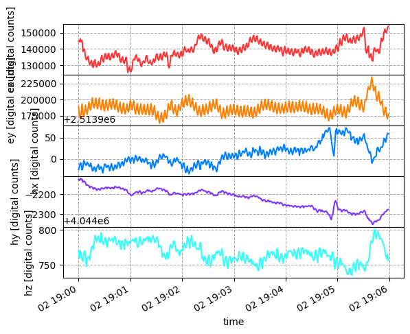
Calibrate Run
[23]:
calibrated_run = run_from_reference.calibrate()
calibrated_run.plot()
[23]:
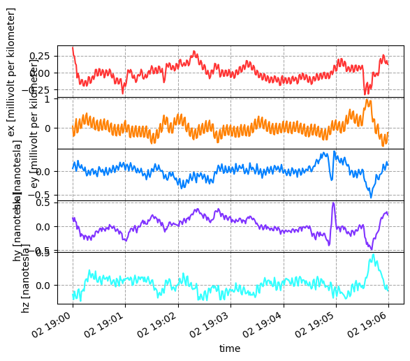
Load Transfer Functions
You can download the transfer functions for CAS04 and NVR08 from IRIS SPUD EMTF. This has already been done as EMTF XML format and will be loaded here.
[24]:
cas04_tf = r"USMTArray.CAS04.2020.xml"
nvr08_tf = r"USMTArray.NVR08.2020.xml"
[25]:
from mt_metadata.transfer_functions.core import TF
[26]:
for tf_fn in [cas04_tf, nvr08_tf]:
    tf_obj = TF(tf_fn)
    tf_obj.read()
    mth5_object.add_transfer_function(tf_obj)
2024-08-09T17:28:37.142425-0700 | WARNING | mt_metadata.transfer_functions.io.emtfxml.metadata.helpers | _read_element | No declination in EMTF XML
2024-08-09T17:28:37.565689-0700 | INFO | mt_metadata.timeseries.filters.filtered | _check_consistency | Assuming all filters have been applied as True
2024-08-09T17:28:37.567595-0700 | INFO | mt_metadata.timeseries.filters.filtered | _check_consistency | Assuming all filters have been applied as True
2024-08-09T17:28:37.569507-0700 | INFO | mt_metadata.timeseries.filters.filtered | _check_consistency | Assuming all filters have been applied as True
2024-08-09T17:28:37.571302-0700 | INFO | mt_metadata.timeseries.filters.filtered | _check_consistency | Assuming all filters have been applied as True
2024-08-09T17:28:37.573091-0700 | INFO | mt_metadata.timeseries.filters.filtered | _check_consistency | Assuming all filters have been applied as True
2024-08-09T17:28:37.603286-0700 | INFO | mt_metadata.timeseries.filters.filtered | _check_consistency | Assuming all filters have been applied as True
2024-08-09T17:28:37.606324-0700 | INFO | mt_metadata.timeseries.filters.filtered | _check_consistency | Assuming all filters have been applied as True
2024-08-09T17:28:37.607961-0700 | INFO | mt_metadata.timeseries.filters.filtered | _check_consistency | Assuming all filters have been applied as True
2024-08-09T17:28:37.609585-0700 | INFO | mt_metadata.timeseries.filters.filtered | _check_consistency | Assuming all filters have been applied as True
2024-08-09T17:28:37.611261-0700 | INFO | mt_metadata.timeseries.filters.filtered | _check_consistency | Assuming all filters have been applied as True
2024-08-09T17:28:37.638728-0700 | INFO | mt_metadata.timeseries.filters.filtered | _check_consistency | Assuming all filters have been applied as True
2024-08-09T17:28:37.640758-0700 | INFO | mt_metadata.timeseries.filters.filtered | _check_consistency | Assuming all filters have been applied as True
2024-08-09T17:28:37.642486-0700 | INFO | mt_metadata.timeseries.filters.filtered | _check_consistency | Assuming all filters have been applied as True
2024-08-09T17:28:37.644142-0700 | INFO | mt_metadata.timeseries.filters.filtered | _check_consistency | Assuming all filters have been applied as True
2024-08-09T17:28:37.645798-0700 | INFO | mt_metadata.timeseries.filters.filtered | _check_consistency | Assuming all filters have been applied as True
2024-08-09T17:28:37.677503-0700 | INFO | mt_metadata.timeseries.filters.filtered | _check_consistency | Assuming all filters have been applied as True
2024-08-09T17:28:37.679475-0700 | INFO | mt_metadata.timeseries.filters.filtered | _check_consistency | Assuming all filters have been applied as True
2024-08-09T17:28:37.681177-0700 | INFO | mt_metadata.timeseries.filters.filtered | _check_consistency | Assuming all filters have been applied as True
2024-08-09T17:28:37.683713-0700 | INFO | mt_metadata.timeseries.filters.filtered | _check_consistency | Assuming all filters have been applied as True
2024-08-09T17:28:37.686350-0700 | INFO | mt_metadata.timeseries.filters.filtered | _check_consistency | Assuming all filters have been applied as True
2024-08-09T17:28:38.183967-0700 | INFO | mt_metadata.timeseries.filters.filtered | _check_consistency | Assuming all filters have been applied as True
2024-08-09T17:28:38.185922-0700 | INFO | mt_metadata.timeseries.filters.filtered | _check_consistency | Assuming all filters have been applied as True
2024-08-09T17:28:38.187754-0700 | INFO | mt_metadata.timeseries.filters.filtered | _check_consistency | Assuming all filters have been applied as True
2024-08-09T17:28:38.189434-0700 | INFO | mt_metadata.timeseries.filters.filtered | _check_consistency | Assuming all filters have been applied as True
2024-08-09T17:28:38.191123-0700 | INFO | mt_metadata.timeseries.filters.filtered | _check_consistency | Assuming all filters have been applied as True
2024-08-09T17:28:38.219756-0700 | INFO | mt_metadata.timeseries.filters.filtered | _check_consistency | Assuming all filters have been applied as True
2024-08-09T17:28:38.221785-0700 | INFO | mt_metadata.timeseries.filters.filtered | _check_consistency | Assuming all filters have been applied as True
2024-08-09T17:28:38.223544-0700 | INFO | mt_metadata.timeseries.filters.filtered | _check_consistency | Assuming all filters have been applied as True
2024-08-09T17:28:38.225615-0700 | INFO | mt_metadata.timeseries.filters.filtered | _check_consistency | Assuming all filters have been applied as True
2024-08-09T17:28:38.227277-0700 | INFO | mt_metadata.timeseries.filters.filtered | _check_consistency | Assuming all filters have been applied as True
2024-08-09T17:28:38.255627-0700 | INFO | mt_metadata.timeseries.filters.filtered | _check_consistency | Assuming all filters have been applied as True
2024-08-09T17:28:38.257764-0700 | INFO | mt_metadata.timeseries.filters.filtered | _check_consistency | Assuming all filters have been applied as True
2024-08-09T17:28:38.260630-0700 | INFO | mt_metadata.timeseries.filters.filtered | _check_consistency | Assuming all filters have been applied as True
2024-08-09T17:28:38.263157-0700 | INFO | mt_metadata.timeseries.filters.filtered | _check_consistency | Assuming all filters have been applied as True
2024-08-09T17:28:38.265648-0700 | INFO | mt_metadata.timeseries.filters.filtered | _check_consistency | Assuming all filters have been applied as True
2024-08-09T17:28:38.300711-0700 | INFO | mt_metadata.timeseries.filters.filtered | _check_consistency | Assuming all filters have been applied as True
2024-08-09T17:28:38.302755-0700 | INFO | mt_metadata.timeseries.filters.filtered | _check_consistency | Assuming all filters have been applied as True
2024-08-09T17:28:38.304607-0700 | INFO | mt_metadata.timeseries.filters.filtered | _check_consistency | Assuming all filters have been applied as True
2024-08-09T17:28:38.306361-0700 | INFO | mt_metadata.timeseries.filters.filtered | _check_consistency | Assuming all filters have been applied as True
2024-08-09T17:28:38.308117-0700 | INFO | mt_metadata.timeseries.filters.filtered | _check_consistency | Assuming all filters have been applied as True
2024-08-09T17:28:38.433515-0700 | INFO | mt_metadata.timeseries.filters.filtered | _check_consistency | Assuming all filters have been applied as True
2024-08-09T17:28:38.435440-0700 | INFO | mt_metadata.timeseries.filters.filtered | _check_consistency | Assuming all filters have been applied as True
2024-08-09T17:28:38.437047-0700 | INFO | mt_metadata.timeseries.filters.filtered | _check_consistency | Assuming all filters have been applied as True
2024-08-09T17:28:38.438641-0700 | INFO | mt_metadata.timeseries.filters.filtered | _check_consistency | Assuming all filters have been applied as True
2024-08-09T17:28:38.440278-0700 | INFO | mt_metadata.timeseries.filters.filtered | _check_consistency | Assuming all filters have been applied as True
2024-08-09T17:28:38.470282-0700 | INFO | mt_metadata.timeseries.filters.filtered | _check_consistency | Assuming all filters have been applied as True
2024-08-09T17:28:38.473730-0700 | INFO | mt_metadata.timeseries.filters.filtered | _check_consistency | Assuming all filters have been applied as True
2024-08-09T17:28:38.475966-0700 | INFO | mt_metadata.timeseries.filters.filtered | _check_consistency | Assuming all filters have been applied as True
2024-08-09T17:28:38.477711-0700 | INFO | mt_metadata.timeseries.filters.filtered | _check_consistency | Assuming all filters have been applied as True
2024-08-09T17:28:38.479501-0700 | INFO | mt_metadata.timeseries.filters.filtered | _check_consistency | Assuming all filters have been applied as True
2024-08-09T17:28:38.509235-0700 | INFO | mt_metadata.timeseries.filters.filtered | _check_consistency | Assuming all filters have been applied as True
2024-08-09T17:28:38.511225-0700 | INFO | mt_metadata.timeseries.filters.filtered | _check_consistency | Assuming all filters have been applied as True
2024-08-09T17:28:38.512832-0700 | INFO | mt_metadata.timeseries.filters.filtered | _check_consistency | Assuming all filters have been applied as True
2024-08-09T17:28:38.514758-0700 | INFO | mt_metadata.timeseries.filters.filtered | _check_consistency | Assuming all filters have been applied as True
2024-08-09T17:28:38.516791-0700 | INFO | mt_metadata.timeseries.filters.filtered | _check_consistency | Assuming all filters have been applied as True
2024-08-09T17:28:38.875697-0700 | INFO | mt_metadata.timeseries.filters.filtered | _check_consistency | Assuming all filters have been applied as True
2024-08-09T17:28:38.877630-0700 | INFO | mt_metadata.timeseries.filters.filtered | _check_consistency | Assuming all filters have been applied as True
2024-08-09T17:28:38.879557-0700 | INFO | mt_metadata.timeseries.filters.filtered | _check_consistency | Assuming all filters have been applied as True
2024-08-09T17:28:38.881263-0700 | INFO | mt_metadata.timeseries.filters.filtered | _check_consistency | Assuming all filters have been applied as True
2024-08-09T17:28:38.883010-0700 | INFO | mt_metadata.timeseries.filters.filtered | _check_consistency | Assuming all filters have been applied as True
2024-08-09T17:28:38.913166-0700 | INFO | mt_metadata.timeseries.filters.filtered | _check_consistency | Assuming all filters have been applied as True
2024-08-09T17:28:38.917754-0700 | INFO | mt_metadata.timeseries.filters.filtered | _check_consistency | Assuming all filters have been applied as True
2024-08-09T17:28:38.920994-0700 | INFO | mt_metadata.timeseries.filters.filtered | _check_consistency | Assuming all filters have been applied as True
2024-08-09T17:28:38.924140-0700 | INFO | mt_metadata.timeseries.filters.filtered | _check_consistency | Assuming all filters have been applied as True
2024-08-09T17:28:38.927140-0700 | INFO | mt_metadata.timeseries.filters.filtered | _check_consistency | Assuming all filters have been applied as True
2024-08-09T17:28:38.961575-0700 | INFO | mt_metadata.timeseries.filters.filtered | _check_consistency | Assuming all filters have been applied as True
2024-08-09T17:28:38.963948-0700 | INFO | mt_metadata.timeseries.filters.filtered | _check_consistency | Assuming all filters have been applied as True
2024-08-09T17:28:38.966380-0700 | INFO | mt_metadata.timeseries.filters.filtered | _check_consistency | Assuming all filters have been applied as True
2024-08-09T17:28:38.968561-0700 | INFO | mt_metadata.timeseries.filters.filtered | _check_consistency | Assuming all filters have been applied as True
2024-08-09T17:28:38.970435-0700 | INFO | mt_metadata.timeseries.filters.filtered | _check_consistency | Assuming all filters have been applied as True
2024-08-09T17:28:39.425273-0700 | INFO | mt_metadata.timeseries.filters.filtered | _check_consistency | Assuming all filters have been applied as True
2024-08-09T17:28:39.427186-0700 | INFO | mt_metadata.timeseries.filters.filtered | _check_consistency | Assuming all filters have been applied as True
2024-08-09T17:28:39.429122-0700 | INFO | mt_metadata.timeseries.filters.filtered | _check_consistency | Assuming all filters have been applied as True
2024-08-09T17:28:39.430845-0700 | INFO | mt_metadata.timeseries.filters.filtered | _check_consistency | Assuming all filters have been applied as True
2024-08-09T17:28:39.432488-0700 | INFO | mt_metadata.timeseries.filters.filtered | _check_consistency | Assuming all filters have been applied as True
2024-08-09T17:28:39.460659-0700 | INFO | mt_metadata.timeseries.filters.filtered | _check_consistency | Assuming all filters have been applied as True
2024-08-09T17:28:39.463400-0700 | INFO | mt_metadata.timeseries.filters.filtered | _check_consistency | Assuming all filters have been applied as True
2024-08-09T17:28:39.465492-0700 | INFO | mt_metadata.timeseries.filters.filtered | _check_consistency | Assuming all filters have been applied as True
2024-08-09T17:28:39.467726-0700 | INFO | mt_metadata.timeseries.filters.filtered | _check_consistency | Assuming all filters have been applied as True
2024-08-09T17:28:39.469988-0700 | INFO | mt_metadata.timeseries.filters.filtered | _check_consistency | Assuming all filters have been applied as True
2024-08-09T17:28:39.499252-0700 | INFO | mt_metadata.timeseries.filters.filtered | _check_consistency | Assuming all filters have been applied as True
2024-08-09T17:28:39.501477-0700 | INFO | mt_metadata.timeseries.filters.filtered | _check_consistency | Assuming all filters have been applied as True
2024-08-09T17:28:39.503187-0700 | INFO | mt_metadata.timeseries.filters.filtered | _check_consistency | Assuming all filters have been applied as True
2024-08-09T17:28:39.504802-0700 | INFO | mt_metadata.timeseries.filters.filtered | _check_consistency | Assuming all filters have been applied as True
2024-08-09T17:28:39.506453-0700 | INFO | mt_metadata.timeseries.filters.filtered | _check_consistency | Assuming all filters have been applied as True
2024-08-09T17:28:39.536022-0700 | INFO | mt_metadata.timeseries.filters.filtered | _check_consistency | Assuming all filters have been applied as True
2024-08-09T17:28:39.538051-0700 | INFO | mt_metadata.timeseries.filters.filtered | _check_consistency | Assuming all filters have been applied as True
2024-08-09T17:28:39.540116-0700 | INFO | mt_metadata.timeseries.filters.filtered | _check_consistency | Assuming all filters have been applied as True
2024-08-09T17:28:39.541830-0700 | INFO | mt_metadata.timeseries.filters.filtered | _check_consistency | Assuming all filters have been applied as True
2024-08-09T17:28:39.543512-0700 | INFO | mt_metadata.timeseries.filters.filtered | _check_consistency | Assuming all filters have been applied as True
2024-08-09T17:28:39.807823-0700 | INFO | mt_metadata.timeseries.filters.filtered | _check_consistency | Assuming all filters have been applied as True
2024-08-09T17:28:39.809733-0700 | INFO | mt_metadata.timeseries.filters.filtered | _check_consistency | Assuming all filters have been applied as True
2024-08-09T17:28:39.811625-0700 | INFO | mt_metadata.timeseries.filters.filtered | _check_consistency | Assuming all filters have been applied as True
2024-08-09T17:28:39.813266-0700 | INFO | mt_metadata.timeseries.filters.filtered | _check_consistency | Assuming all filters have been applied as True
2024-08-09T17:28:39.814940-0700 | INFO | mt_metadata.timeseries.filters.filtered | _check_consistency | Assuming all filters have been applied as True
2024-08-09T17:28:39.843059-0700 | INFO | mt_metadata.timeseries.filters.filtered | _check_consistency | Assuming all filters have been applied as True
2024-08-09T17:28:39.845268-0700 | INFO | mt_metadata.timeseries.filters.filtered | _check_consistency | Assuming all filters have been applied as True
2024-08-09T17:28:39.847315-0700 | INFO | mt_metadata.timeseries.filters.filtered | _check_consistency | Assuming all filters have been applied as True
2024-08-09T17:28:39.849990-0700 | INFO | mt_metadata.timeseries.filters.filtered | _check_consistency | Assuming all filters have been applied as True
2024-08-09T17:28:39.851889-0700 | INFO | mt_metadata.timeseries.filters.filtered | _check_consistency | Assuming all filters have been applied as True
2024-08-09T17:28:39.889154-0700 | INFO | mt_metadata.timeseries.filters.filtered | _check_consistency | Assuming all filters have been applied as True
2024-08-09T17:28:39.892432-0700 | INFO | mt_metadata.timeseries.filters.filtered | _check_consistency | Assuming all filters have been applied as True
2024-08-09T17:28:39.895193-0700 | INFO | mt_metadata.timeseries.filters.filtered | _check_consistency | Assuming all filters have been applied as True
2024-08-09T17:28:39.897730-0700 | INFO | mt_metadata.timeseries.filters.filtered | _check_consistency | Assuming all filters have been applied as True
2024-08-09T17:28:39.900407-0700 | INFO | mt_metadata.timeseries.filters.filtered | _check_consistency | Assuming all filters have been applied as True
Have a look at the transfer function summary
[27]:
mth5_object.tf_summary.summarize()
tf_df = mth5_object.tf_summary.to_dataframe()
tf_df
[27]:
| station | survey | latitude | longitude | elevation | tf_id | units | has_impedance | has_tipper | has_covariance | period_min | period_max | hdf5_reference | station_hdf5_reference | |
|---|---|---|---|---|---|---|---|---|---|---|---|---|---|---|
| 0 | CAS04 | CONUS_South | 37.633351 | -121.468382 | 329.387 | CAS04 | none | True | True | True | 4.65455 | 29127.11 | <HDF5 object reference> | <HDF5 object reference> |
| 1 | NVR08 | CONUS_South | 38.326630 | -118.082382 | 1375.425 | NVR08 | none | True | True | True | 4.65455 | 29127.11 | <HDF5 object reference> | <HDF5 object reference> |
Plot the transfer functions using MTpy
Note: This currently works on branch mtpy-v2_plots
For another curated example of TF plotting, see this example in the mtpy-v2 repository.
[28]:
# # Skip this step if mtpy already installed
# !pip install mtpy-v2
[29]:
# from mtpy import MTCollection
[30]:
# mc = MTCollection()
# mc.open_collection(r"8P_CAS04_NVR08")
[31]:
# mc.dataframe
[32]:
# mc.plot_mt_response?
[33]:
# pmr = mc.plot_mt_response(["CAS04", "NVR08"], survey="CONUS_South", plot_style="compare")
Plot Station locations
Here we can plot station locations for all stations in the file, or we can give it a bounding box. If you have internet access a basemap will be plotted using Contextily.
[34]:
# st = mc.plot_stations(pad=.9, fig_num=5, fig_size=[6, 4])
[35]:
# st.fig.get_axes()[0].set_xlim((-121.9, -117.75))
# st.fig.get_axes()[0].set_ylim((37.35, 38.5))
# st.update_plot()
[36]:
# mth5_object.close_mth5()