Filters

This section includes information about filters, which can be a very painful process and somewhat obtuse.

Filters are basically anything that manipulates the time series data into something else. This includes scaling, removing instrument response, removing trends, notch filtering, passband filtering, etc. We want to work with data that is in physical units, but the data are often collected in digital counts. To transform between the two we need to apply or unapply certain filters. When going from physical units to digital counts we are applying filters, channel_metadata.filter.applied = [True], whereas going from counts to physical units we are unapplying the filters channel_metadata.filter.applied = [False]. This may seem backwards, but this is the way most archived data is thought of. Then any filter applied to physical units for the purposes of cleaning the data are channel_metadata.filter.applied = [True].

Note: currently there are not tools to convert digital counts to physical units, this is a work in progress. Nevertheless all the information is there for you to do the transformation.

Supported filters in mt_metadata.timeseries.filters are:

Filter	Description
CoefficientFilter	A coefficient filter scales the data by a given factor, a real value.
FIRFilter	A finite impulse response filter is commonly an anti-alias filter and is represented as a 1-D array of real valued coefficients.
PoleZeroFilter	A pole-zero filter is often an type of bandpass filter. It is represented as symmetric complex poles and zeros with a scale factor
TimeDelayFilter	A time delay filter delays the data by a real valued time delay. A negative value is a delay and a positive value is a prediction.
FrequencyResponseTableFilter	A frequency, amplitude, phase look-up table, commonly in physical units and degrees. This is commonly how manufacturers provide instrument responses.
ChannelResponseFilter	A comprehensive representation of all filters. Contains a list of all filters, should be the most commonly used filter object as it can compute the total response, and estimate the passband and normalization frequency.

Filter Base

All filters inherit from a FilterBase class, which has attributes and methods common to all filters.

Units

The two common to all filters are units_in and units_out. These attributes are key as they describes how the filters are transforming the data. The units should be SI units and given as all lowercase full names. For example Volts would be volts and V/m would be volts per meter. All units are represented in short form.

Complex Response

A method is provided to compute the complex response, this is slightly different for each filter and the method overwritten by the different filters.

Pass Band

A method is also provided to compute the “pass band” of a given filter. This is the band where the response is flat, the estimation is only approximate and should be used with caution. It works well for simple filters, but more complex filters, it tries to pick the longest segment with a flat response. CoefficientFilter and TimeDelayFilter objects have an infinite pass band. FrequencyResponseTableFilter estimate the pass band within the given frequencies, unless told otherwise. If the frequency range is out of the range of the calibration frequencies extrapolation is applied. This should also be done with caution.

[1]:

%matplotlib inline
import numpy as np

# make a general frequency array to calculate complex response
# note that these are linear frequencies and the complex response uses angular frequencies
frequencies = np.logspace(-5, 5, 500)

Coefficient Filter

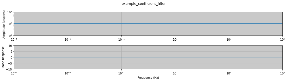
A coefficient filter is relatively simple. It includes a scale factor represented as gain.

[2]:

from mt_metadata.timeseries.filters import CoefficientFilter

[3]:

cf = CoefficientFilter(units_in="volts", units_out="V", gain=100.0, name="example_coefficient_filter")
cf

[3]:

{
    "coefficient_filter": {
        "calibration_date": "1980-01-01",
        "gain": 100.0,
        "name": "example_coefficient_filter",
        "type": "coefficient",
        "units_in": "V",
        "units_out": "V"
    }
}

[4]:

cf.plot_response(frequencies, x_units="frequency")

../../_images/examples_notebooks_filters_example_6_0.png

FIR Filter

An finite impulse response filter is commonly used as an anti-alias filter, and is represented as a 1-D array of real valued coefficients.

[5]:

from mt_metadata.timeseries.filters import FIRFilter

[6]:

fir = FIRFilter(
    units_in="volts",
    units_out="volts",
    name="example_fir",
    decimation_input_sample_rate=32000,
    gain=0.999904,
    symmetry="EVEN",
    decimation_factor=16,
)

fir.coefficients = [
    1.0828314e-06, 1.7808272e-06, 3.2410387e-06, 5.4627321e-06, 8.682945e-06, 1.3240843e-05, 1.9565294e-05,
    2.8185128e-05, 3.9656901e-05, 5.4688699e-05, 7.4153548e-05, 9.8989171e-05, 0.00013036761, 0.00016954952,
    0.00021798223, 0.00027731725, 0.00034936491, 0.00043613836, 0.00053984317, 0.0006628664, 0.00080777059,
    0.00097733398, 0.0011744311, 0.0014021378, 0.0016635987, 0.0019620692, 0.0023008469, 0.0026832493,
    0.0031125348, 0.0035918986, 0.0041243695, 0.0047127693, 0.0053596641, 0.0060672448, 0.0068373145,
    0.0076711699, 0.0085695535, 0.0095325625, 0.010559602, 0.01164928, 0.012799387, 0.014006814, 0.015267504,
    0.016576445, 0.017927598, 0.019313928, 0.020727372, 0.022158878, 0.023598416, 0.025035053, 0.026456987,
    0.027851671, 0.029205887, 0.030505868, 0.031737458, 0.032886244, 0.03393773, 0.034877509, 0.035691477,
    0.036365997, 0.036888145, 0.037245877, 0.03742826, 0.037425674, 0.03723, 0.036834806, 0.036235519,
    0.035429578, 0.034416564, 0.033198304, 0.031778947, 0.030165028, 0.028365461, 0.026391543, 0.024256891,
    0.021977346, 0.019570865, 0.017057346, 0.014458441, 0.011797323, 0.009098433, 0.0063871844, 0.0036896705,
    0.0010323179, -0.0015584482, -0.0040565561, -0.0064366534, -0.0086744577, -0.010747112, -0.012633516,
    -0.014314661, -0.0157739, -0.01699724, -0.017973563, -0.018694809, -0.019156145, -0.01935605, -0.019296378,
    -0.018982368, -0.018422581, -0.017628808, -0.016615927, -0.015401681, -0.014006456, -0.012452973,
    -0.010765962, -0.0089718029, -0.0070981304, -0.0051734182, -0.0032265538, -0.0012863991, 0.0006186511,
    0.0024610918, 0.0042147399, 0.0058551184, 0.0073598339, 0.0087089101, 0.0098850802, 0.01087404, 0.011664648,
    0.012249067, 0.012622863, 0.012785035, 0.012737988, 0.012487462, 0.01204238, 0.011414674, 0.010619033,
    0.0096726287, 0.0085947802, 0.007406604, 0.006130626, 0.0047903718, 0.0034099557, 0.002013647, 0.00062545808,
    -0.0007312728, -0.0020342721, -0.0032627005, -0.0043974896, -0.0054216445, -0.0063205026, -0.0070819431,
    -0.0076965573, -0.0081577515, -0.0084618134, -0.0086079109, -0.0085980454, -0.0084369555, -0.0081319623,
    -0.0076927822, -0.0071312929, -0.0064612622, -0.005698049, -0.0048582871, -0.0039595389, -0.0030199524,
    -0.0020579058, -0.0010916605, -0.00013902181, 0.00078298012, 0.0016583927, 0.0024726097, 0.0032126096,
    0.0038671608, 0.0044269804, 0.0048848582, 0.005235733, 0.0054767267, 0.0056071337, 0.0056283739,
    0.0055438946, 0.0053590466, 0.0050809216, 0.0047181565, 0.0042807218, 0.0037796798, 0.0032269375,
    0.0026349833, 0.0020166242, 0.001384723, 0.00075194426, 0.00013050952, -0.00046802824, -0.0010329896,
    -0.0015547526, -0.0020249044, -0.0024363673, -0.0027834927, -0.0030621202, -0.0032696081, -0.0034048304,
    -0.003468141, -0.0034613123, -0.003387446, -0.0032508562, -0.003056939, -0.0028120177, -0.0025231787,
    -0.0021980959, -0.0018448512, -0.001471751, -0.0010871479, -0.00069926586, -0.00031603608, 5.5052958e-05,
    0.00040709358, 0.00073387625, 0.0010299878, 0.0012908906, 0.0015129783, 0.0016936094, 0.0018311206,
    0.0019248178, 0.0019749457, 0.0019826426, 0.0019498726, 0.0018793481, 0.001774437, 0.0016390601,
    0.0014775817, 0.0012946966, 0.0010953132, 0.00088443852, 0.00066706788, 0.00044807568, 0.00023212004,
    2.3551687e-05, -0.00017366471, -0.00035601447, -0.00052048819, -0.00066461961, -0.0007865114, -0.00088484585,
    -0.00095888576, -0.0010084547, -0.0010339168, -0.0010361352, -0.0010164281, -0.00097651512, -0.0009184563,
    -0.00084458862, -0.00075745879, -0.00065975531, -0.0005542388, -0.00044368068, -0.00033079527, -0.00021818698,
    -0.0001082966, -3.3548122e-06, 9.4652831e-05, 0.00018401834, 0.00026333242, 0.00033149892, 0.00038773834,
    0.00043159194, 0.00046290434, 0.0004818163, 0.0004887383, 0.00048432534, 0.00046944799, 0.00044515711,
    0.0004126484, 0.0003732258, 0.00032826542, 0.0002791743, 0.00022736372, 0.0001742071, 0.00012101705,
    6.9016627e-05, 1.9314915e-05, -2.7108661e-05, -6.9420195e-05, -0.00010694123, -0.00013915499, -0.00016570302,
    -0.00018639189, -0.00020117435, -0.00021015058, -0.00021354953, -0.00021171506, -0.00020509114, -0.00019420317,
    -0.00017963824, -0.00016202785, -0.00014203126, -0.00012030972, -9.7522447e-05, -7.4297881e-05, -5.1229126e-05,
    -2.8859566e-05, -7.6714587e-06, 1.191924e-05, 2.9567975e-05, 4.5006156e-05, 5.8043028e-05, 6.8557049e-05,
    7.6507284e-05, 8.1911501e-05, 8.4854546e-05, 8.5473977e-05, 8.3953237e-05, 8.0514517e-05, 7.5410928e-05,
    6.8914269e-05, 6.1308667e-05, 5.2886291e-05, 4.3926615e-05, 3.4708195e-05, 2.5484322e-05, 1.6489239e-05,
    7.9309229e-06, -1.335887e-08, -7.1985955e-06, -1.3510014e-05, -1.8867066e-05, -2.32245e-05, -2.6558888e-05,
    -2.8887769e-05, -3.0242758e-05, -3.0684769e-05, -3.0291432e-05, -2.9154804e-05, -2.7376906e-05, -2.5070442e-05,
    -2.2347936e-05, -1.9321938e-05, -1.6109379e-05, -1.2808429e-05, -9.5234091e-06, -6.3382245e-06,
    -3.3291028e-06, -5.5987789e-07, 1.9187619e-06, 4.072373e-06, 5.8743913e-06, 7.312286e-06, 8.3905516e-06,
    9.10975e-06, 9.4979405e-06, 9.5751602e-06, 9.3762619e-06, 8.9382884e-06, 8.301693e-06, 7.5045982e-06,
    6.592431e-06, 5.6033018e-06, 4.5713236e-06, 3.5404175e-06, 2.5302468e-06, 1.5771827e-06, 6.9930724e-07,
    -8.6047464e-08, -7.6676685e-07, -1.3332562e-06, -1.7875625e-06, -2.1266892e-06, -2.35267e-06, -2.4824365e-06,
    -2.5098916e-06, -2.4598471e-06, -2.335345e-06, -2.1523615e-06, -1.9251499e-06, -1.6707684e-06, -1.3952398e-06,
    -1.1173763e-06, -8.4543007e-07, -5.7948262e-07, -3.444687e-07, -1.2505329e-07, 6.1743521e-08, 2.1873758e-07,
    3.4424812e-07, 4.3748074e-07, 4.931357e-07, 5.2551894e-07, 5.344753e-07, 5.136161e-07, 4.9029785e-07,
    4.3492003e-07, 3.8198567e-07, 3.2236682e-07, 2.6023093e-07, 1.9363162e-07, 1.3382508e-07, 6.8672463e-08,
    2.1443693e-08, -1.9671351e-09, -4.7522178e-08, -6.2719053e-08, -1.0190665e-07, -1.2015286e-07, -1.103657e-07,
    -1.0294882e-07, -1.1965994e-07, -1.3612285e-07, -1.463918e-07, -1.4752351e-07, 3.9802276e-07]

[7]:

fir.plot_response(frequencies, x_units="frequency", pb_tol=.5)
print(f"Pass Band frequency range estimation: {fir.pass_band(frequencies, tol=.5)}")

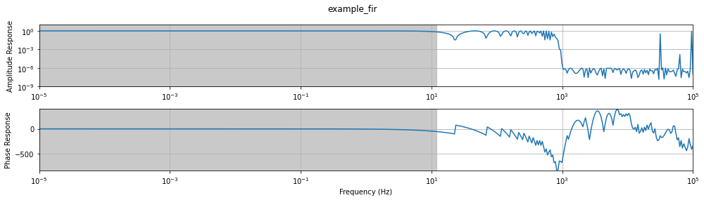
../../_images/examples_notebooks_filters_example_10_0.png

Pass Band frequency range estimation: [1.00000000e-05 1.18071285e+01]

Pole Zero Filter

A pole-zero filter is a mathematical way to represent a filter using complex valued poles and zeros and a scaling factor. The advantage of the pole-zero representation is that arbitrary frequency ranges can be computed without having to extrapolate.

[8]:

from mt_metadata.timeseries.filters import PoleZeroFilter

[9]:

pz = PoleZeroFilter(units_in="volts", units_out="nanotesla", name="example_zpk_response")
pz.poles = [(-6.283185+10.882477j), (-6.283185-10.882477j), (-12.566371+0j)]
pz.zeros = []
pz.normalization_factor = 2002.269
pz

[9]:

{
    "pole_zero_filter": {
        "calibration_date": "1980-01-01",
        "gain": 1.0,
        "name": "example_zpk_response",
        "normalization_factor": 2002.269,
        "poles": {
            "real": [
                -6.283185,
                -6.283185,
                -12.566371
            ],
            "imag": [
                10.882477,
                -10.882477,
                0.0
            ]
        },
        "type": "zpk",
        "units_in": "V",
        "units_out": "nT",
        "zeros": {
            "real": [],
            "imag": []
        }
    }
}

[10]:

pz.plot_response(frequencies, x_units="frequency", pb_tol=1e-2)
print(f"Pass Band frequency range estimation: {pz.pass_band(frequencies, tol=1e-2)}")

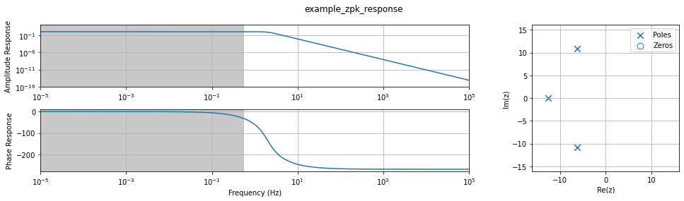
../../_images/examples_notebooks_filters_example_14_0.png

Pass Band frequency range estimation: [1.00000000e-05 5.36363132e-01]

Time Delay Filter

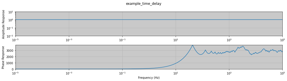
A time delay filter are often incorporated in the AD converter that controls mulitple channels and creates a small time delay as it shifts between the channels. A positive value predicts time and a negative value delays time. For causality the value should always be negative. The delay is givne in seconds.

[11]:

from mt_metadata.timeseries.filters import TimeDelayFilter

[12]:

td = TimeDelayFilter(units_in="volts", units_out="volts", name="example_time_delay", delay=-.25)
td.pass_band(frequencies)

[12]:

array([1.e-05, 1.e+05])

[13]:

td.plot_response(frequencies, x_units="frequency")

../../_images/examples_notebooks_filters_example_18_0.png

FrequencyResponseTableFilter

Commonly to calibrate the frequency response of an instrument a manufacturer will run a calibration taking measurements at discrete frequencies and then supplying a table of frequency, amplitude, and phase for the users. This is more accurate than pole-zero representation but has limitations in that extrapolation needs to be applied to frequencies outside of the calibrated frequencies and interpolation between calibrated frequencies.

Note: phase is assumed to be in radians.

[14]:

from mt_metadata.timeseries.filters import FrequencyResponseTableFilter

[15]:

fap = FrequencyResponseTableFilter(units_in="volts", units_out="nanotesla", name="example_fap")

fap.frequencies = [
95312000e-03,   2.76214000e-03,   3.90625000e-03,
52427000e-03,   7.81250000e-03,   1.10485000e-02,
56250000e-02,   2.20971000e-02,   3.12500000e-02,
41942000e-02,   6.25000000e-02,   8.83883000e-02,
25000000e-01,   1.76780000e-01,   2.50000000e-01,
53550000e-01,   5.00000000e-01,   7.07110000e-01,
00000000e+00,   1.41420000e+00,   2.00000000e+00,
82840000e+00,   4.00000000e+00,   5.65690000e+00,
00000000e+00,   1.13140000e+01,   1.60000000e+01,
26270000e+01,   3.20000000e+01,   4.52550000e+01,
40000000e+01,   9.05100000e+01,   1.28000000e+02,
81020000e+02,   2.56000000e+02,   3.62040000e+02,
12000000e+02,   7.24080000e+02,   1.02400000e+03,
44820000e+03,   2.04800000e+03,   2.89630000e+03,
09600000e+03,   5.79260000e+03,   8.19200000e+03,
15850000e+04]

fap.amplitudes = [
59009000e-03,   3.07497000e-03,   5.52793000e-03,
47448000e-03,   1.54565000e-02,   2.49498000e-02,
96462000e-02,   7.87192000e-02,   1.57134000e-01,
09639000e-01,   5.94224000e-01,   1.12698000e+00,
01092000e+00,   3.33953000e+00,   5.00280000e+00,
62396000e+00,   7.97545000e+00,   8.82872000e+00,
36883000e+00,   9.64102000e+00,   9.79664000e+00,
87183000e+00,   9.90666000e+00,   9.92845000e+00,
93559000e+00,   9.93982000e+00,   9.94300000e+00,
93546000e+00,   9.93002000e+00,   9.90873000e+00,
86383000e+00,   9.78129000e+00,   9.61814000e+00,
26461000e+00,   8.60175000e+00,   7.18337000e+00,
46123000e+00,  -8.72600000e-01,  -5.15684000e+00,
    -2.95111000e+00,  -9.28512000e-01,  -2.49850000e-01,
    -5.75682000e-02,  -1.34293000e-02,  -1.02708000e-03,
09577000e-03]

fap.phases = [
60824000e-02,   1.09174000e-01,   1.56106000e-01,
22371000e-01,   3.12020000e-01,   4.41080000e-01,
23548000e-01,   8.77188000e-01,   1.23360000e+00,
71519000e+00,   2.35172000e+00,   3.13360000e+00,
98940000e+00,   4.67269000e+00,   4.96593000e+00,
65875000e+00,   3.95441000e+00,   3.11098000e+00,
30960000e+00,   1.68210000e+00,   1.17928000e+00,
20015000e-01,   5.36474000e-01,   3.26955000e-01,
48051000e-01,  -8.24275000e-03,  -1.66064000e-01,
    -3.48852000e-01,  -5.66625000e-01,  -8.62435000e-01,
    -1.25347000e+00,  -1.81065000e+00,  -2.55245000e+00,
    -3.61512000e+00,  -5.00185000e+00,  -6.86158000e+00,
    -8.78698000e+00,  -9.08920000e+00,  -4.22925000e+00,
15533000e-01,   6.00661000e-01,   3.12368000e-01,
31660000e-01,   5.01553000e-02,   1.87239000e-02,
68243000e-03]

[16]:

from matplotlib import pyplot as plt

[17]:

fap.plot_response(frequencies, x_units="frequency", unwrap=True, pb_tol=1E-2, interpolation_method="slinear")
print(f"Pass Band frequency range estimation: {fap.pass_band(fap.frequencies, tol=1e-2,  interpolation_method='slinear')}")

2023-09-27T16:22:20.641040-0700 | WARNING | mt_metadata.timeseries.filters.frequency_response_table_filter | complex_response | Extrapolating, use values outside calibration frequencies with caution
2023-09-27T16:22:20.641040-0700 | WARNING | mt_metadata.timeseries.filters.frequency_response_table_filter | complex_response | Extrapolating, use values outside calibration frequencies with caution

../../_images/examples_notebooks_filters_example_23_1.png

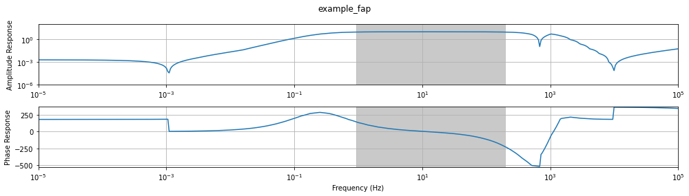
Pass Band frequency range estimation: [  2.   181.02]

IMPORTANT: As you can see above extrapolation is unstable and will have change the data in unknown ways. If you need to extrapolate past the calibrated frequencies try to extrapolate using a different method than the one provided. Try using a different interpolation method, or a different curve fitting algorithm.

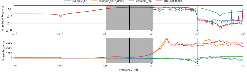
ChannelResponseFilter

These individual filters are useful, but the more practical use is combining all filters into a single filter and calculating the total response. The mt_metadata.timeseries.filters.ChannelResponseFilter is provide for this purpose.

[18]:

from mt_metadata.timeseries.filters import ChannelResponseFilter

[19]:

channel_response = ChannelResponseFilter()
channel_response.filters_list = [fir, td, fap]
channel_response.frequencies = frequencies

[20]:

channel_response.plot_response(x_units="frequency", pb_tol=1e-1, include_delay=True)

2023-09-27T16:22:21.020759-0700 | WARNING | mt_metadata.timeseries.filters.frequency_response_table_filter | complex_response | Extrapolating, use values outside calibration frequencies with caution
2023-09-27T16:22:21.042704-0700 | WARNING | mt_metadata.timeseries.filters.frequency_response_table_filter | complex_response | Extrapolating, use values outside calibration frequencies with caution
2023-09-27T16:22:21.055112-0700 | WARNING | mt_metadata.timeseries.filters.frequency_response_table_filter | complex_response | Extrapolating, use values outside calibration frequencies with caution
2023-09-27T16:22:21.076144-0700 | WARNING | mt_metadata.timeseries.filters.frequency_response_table_filter | complex_response | Extrapolating, use values outside calibration frequencies with caution
2023-09-27T16:22:21.092895-0700 | WARNING | mt_metadata.timeseries.filters.frequency_response_table_filter | complex_response | Extrapolating, use values outside calibration frequencies with caution

../../_images/examples_notebooks_filters_example_28_1.png

Estimate Total Sensitivity

If you want to do a quick calibration you can divide the time series by the total sensitivity and it will be accurate within the pass band.

[21]:

print(f"Normalization Frequency: {channel_response.normalization_frequency} Hz")
print(f"Pass Band: {channel_response.pass_band} Hz")
print(f"Total Sensitivity: {channel_response.compute_instrument_sensitivity(sig_figs=3)}")

2023-09-27T16:22:21.571180-0700 | WARNING | mt_metadata.timeseries.filters.frequency_response_table_filter | complex_response | Extrapolating, use values outside calibration frequencies with caution
2023-09-27T16:22:21.593486-0700 | WARNING | mt_metadata.timeseries.filters.frequency_response_table_filter | complex_response | Extrapolating, use values outside calibration frequencies with caution
Normalization Frequency: 1.097 Hz
2023-09-27T16:22:21.609817-0700 | WARNING | mt_metadata.timeseries.filters.frequency_response_table_filter | complex_response | Extrapolating, use values outside calibration frequencies with caution
Pass Band: [ 0.1018629  11.80712847] Hz
2023-09-27T16:22:21.629781-0700 | WARNING | mt_metadata.timeseries.filters.frequency_response_table_filter | complex_response | Extrapolating, use values outside calibration frequencies with caution
2023-09-27T16:22:21.648280-0700 | WARNING | mt_metadata.timeseries.filters.frequency_response_table_filter | complex_response | Extrapolating, use values outside calibration frequencies with caution
2023-09-27T16:22:21.661262-0700 | WARNING | mt_metadata.timeseries.filters.frequency_response_table_filter | complex_response | Extrapolating, use values outside calibration frequencies with caution
2023-09-27T16:22:21.681687-0700 | WARNING | mt_metadata.timeseries.filters.frequency_response_table_filter | complex_response | Extrapolating, use values outside calibration frequencies with caution
2023-09-27T16:22:21.705189-0700 | WARNING | mt_metadata.timeseries.filters.frequency_response_table_filter | complex_response | Extrapolating, use values outside calibration frequencies with caution
2023-09-27T16:22:21.725088-0700 | WARNING | mt_metadata.timeseries.filters.frequency_response_table_filter | complex_response | Extrapolating, use values outside calibration frequencies with caution
Total Sensitivity: 9.405

Check if units are proper between filters

The output units of the first filter must be the same units as the input units for the second filter. This is done when the filter list is set. Here you can see that the unit order is not correct.

[22]:

channel_response = ChannelResponseFilter()
channel_response.filters_list = [cf, fap, pz]

2023-09-27T16:22:21.747735-0700 | ERROR | mt_metadata.timeseries.filters.channel_response_filter | _check_consistency_of_units | Unit consistency is incorrect. The input units for example_zpk_response should be nT not V

---------------------------------------------------------------------------
ValueError                                Traceback (most recent call last)
~\AppData\Local\Temp\1\ipykernel_19688\4206849502.py in <cell line: 2>()
      1 channel_response = ChannelResponseFilter()
----> 2 channel_response.filters_list = [cf, fap, pz]

~\OneDrive - DOI\Documents\GitHub\mt_metadata\mt_metadata\base\metadata.py in __setattr__(self, name, value)
    360
    361         if name in skip_list:
--> 362             super().__setattr__(name, value)
    363             return
    364         if not name.startswith("_"):

~\OneDrive - DOI\Documents\GitHub\mt_metadata\mt_metadata\timeseries\filters\channel_response_filter.py in filters_list(self, filters_list)
     70         """set the filters list and validate the list"""
     71         self._filters_list = self._validate_filters_list(filters_list)
---> 72         self._check_consistency_of_units()
     73
     74     @property

~\OneDrive - DOI\Documents\GitHub\mt_metadata\mt_metadata\timeseries\filters\channel_response_filter.py in _check_consistency_of_units(self)
    338                     )
    339                     self.logger.error(msg)
--> 340                     raise ValueError(msg)
    341                 previous_units = mt_filter.units_out
    342

ValueError: Unit consistency is incorrect. The input units for example_zpk_response should be nT not V